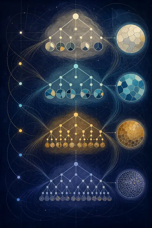
The Logic of Systems of Granular Partitions

We introduce the notation $\backslash mathcal\{EM\}$ and $\backslash mathcal\{RTM\}$ to denote the classes of structures satisfying EM and RTM. We now define granular partitions $x$ as triples of the form

where $Z\; \backslash in\; \backslash mathcal\{RTM\}$ is called the cell tree of the partition, $\backslash Delta\; \backslash in\; \backslash mathcal\{EM\}$ is called the target domain of the partition, and the projection-mapping of signature $\backslash rho\; :\; Z\; \backslash rightarrow\; \backslash Delta$ has the following properties:

In general the $\backslash rho$ will be not an onto mapping due to the selective and granular character of granular partitions.

Consider the tree structures in Figure 2 and the way the corresponding cell trees project onto the object Fred. The labels on the nodes of the tree and the cells are an important aspect of the representations of Fred’s parts. We will interpret the labels of granular partitions as names of the entities the labeled cell projects on. Notice that the label ‘Fred’s left leg’ is not understood as a definite description [Rus19], i.e., the unique instance of the type (class, kind) left human leg that is part of Fred at a given time. This leg keeps its name during its existence. If Fred donates his left leg and the leg becomes a part of Bill then the name the name of Bill’s new leg is still ‘Fred’s left leg’.

Let $\backslash Lambda$ be the set of names in language $\backslash lambda$ and let $(Z,\; \backslash Delta,\; \backslash rho)$ be a granular partition. A labeled granular partition is then a quintuple of the form

which is such that the labeling function $\backslash phi\; :\; \backslash Lambda\; \backslash rightarrow\; Z$ is a one-one and onto mapping, i.e. each cell in the tree $Z$ has a unique label. It follows that if $\backslash lambda\_i\; \backslash in\; \backslash Lambda$ is a label for a cell, then there is an entity in $x\; \backslash in\; \backslash Delta$ such that $\backslash lambda\_i$ is the name of $x$. Names are finite strings of some alphabet $\backslash lambda$. Since a cell tree has finitely many cells, it is always possible to assign finite strings of $\backslash lambda$ to the cells of a given partition. The labeling mappings $\backslash phi$ will in general be partial, since finite partitions do not exhaust all strings of the underlying alphabet.

Consider the left part of Figure 4. The corresponding labeled granular partition $(Z,\; \backslash Delta,\; \backslash rho,\; \backslash alpha,\; \backslash phi)$ has projection and labeling mappings $\backslash rho$ and $\backslash phi$ which are such that the following holds:

Here $\backslash phi(\text{'}Montana\text{'})$ stands for “the cell labeled ‘Montana’” and Montana refers to the targeted portions of reality (in this case, the portion of the surface of Earth that is occupied by the Federal State Montana).

Consider the right part of Figure 4. Here we have a ‘mislabeling’ of the form $\backslash rho(\backslash phi(\backslash text\{\text{'}Idaho\text{'}\}))\; =\; \backslash text\{Montana\}$, which means that the cell labeled ‘Idaho’ projects onto the piece of land which is usually referred to as Montana. Intuitively, this means that the labeling of this partition is in a certain way incompatible with the way the vast majority of other partitions which target the same domain are labeled. In particular, it is incompatible with the way the federal government of the United States labels their maps (which are special kinds of partitions [BS01]).

Let $(Z,\; \backslash Delta,\; \backslash rho)$ be a granular partition and let $\backslash Omega$ be a set of types which together with their instances – objects in $\backslash mathcal\{EM\}$ – satisfy the axioms of our Minimal Type Theory (MTT). A typing for partition $(Z,\; \backslash Delta,\; \backslash rho)$ is a mapping $\backslash psi$ of signature $\backslash psi\; :\; Z\; \backslash rightarrow\; \backslash Omega$ assigning cells in $Z$ to members of the set $\backslash Omega$. If $\backslash psi(z)\; =\; c$ then we say that the cell $z$ is of type $c$. A typed granular partition then is a quintuple of the form

such that the typing function $\backslash psi$ has the following properties:

Consider the left part of Figure 3. The corresponding typed granular partition $(Z,\; \backslash Delta,\; \backslash rho,\; \backslash Omega,\; \backslash psi)$ has projection and typing mappings $\backslash rho$ and $\backslash psi$ which are such that the following holds:

A labeled and typed granular partition then is a seven-tuple of the form

such that $(Z,\; \backslash Delta,\; \backslash rho)$ is a granular partition, $(Z,\; \backslash Delta,\; \backslash rho,\; \backslash Lambda,\; \backslash phi)$ is a labeled granular partition, and $(Z,\; \backslash Delta,\; \backslash rho,\; \backslash Omega,\; \backslash psi)$ is a typed granular partition.

Let $\backslash Pi$ be a set of labeled typed granular partitions. Let $\backslash Gamma\_1\; =\; (Z\_1,\; \backslash Delta\_1,\; \backslash rho\_1,\; \backslash Lambda\_1,\; \backslash phi\_1,\; \backslash Omega\_1,\; \backslash psi\_1)$ and $\backslash Gamma\_2\; =\; (Z\_2,\; \backslash Delta\_2,\; \backslash rho\_2,\; \backslash Lambda\_2,\; \backslash phi\_2,\; \backslash Omega\_2,\; \backslash psi\_2)$ be labeled, typed granular partitions in $\backslash Pi$. And let $\backslash Gamma\_1$ and $\backslash Gamma\_2$ be the labeled, typed granular partitions in Figures 2 and 3. One can see that $\backslash Gamma\_1$ and $\backslash Gamma\_2$ stand in a kind of refinement relation to each other. We will use the symbol $\backslash preceq$ to refer to this relation and write $\backslash Gamma\_1\; \backslash preceq\; \backslash Gamma\_2$ to express the fact that the granular partition $\backslash Gamma\_1$ is a refined by the granular partition $\backslash Gamma\_2$.

We give a formal account of the relation $\backslash preceq$ as follows. For labeled typed granular partitions $\backslash Gamma\_1,\; \backslash Gamma\_2\; \backslash in\; \backslash Pi$ we say that $\backslash Gamma\_1\; \backslash preceq\; \backslash Gamma\_2$ if and only if there exists a mapping $f\; :\; Z\_1\; \backslash rightarrow\; Z\_2$ with the following properties:

The existence of the mapping $f$ with its particular properties (i-v) ensures that if partition $\backslash Gamma\_1$ is a refinement of partition $\backslash Gamma\_2$, then we can map cells in $Z\_1$ to cells in $Z\_2$ in such a way that: (a) if two cells in $z\_i,\; z\_j\; \backslash in\; Z\_1$ are subcells of each other then so are their counterparts in $f(z\_i),\; f(z\_j)\; \backslash in\; Z\_2$; (b) the target $\backslash rho\_1(z)$ of the cell $z\; \backslash in\; Z\_1$ is identical to the target $\backslash rho\_2(f(z))$ of its counterpart $f(z)\; \backslash in\; Z\_2$; (c) the cells $z\; \backslash in\; Z\_1$ and $f(z)\; \backslash in\; Z\_2$ have the same labels; and (d) the cells $z\; \backslash in\; Z\_1$ and $f(z)\; \backslash in\; Z\_2$ have the same type. In other words we require that if partition $\backslash Gamma\_1$ is a refinement of partition $\backslash Gamma\_2$ then there exists an order-, label-, type-, and target-preserving mapping $f$ such that the diagrams in Figure 5 commute.

Let $\backslash Gamma,\; \backslash Gamma\_1,\; \backslash Gamma\_2$ and $\backslash Gamma\_3$ be a labeled, typed granular partitions. We can show that the relation $\backslash preceq$ is reflexive (ref) and transitive (tr):

Consider the left part of Figure 7. We have a partition $\backslash Gamma\_x$ with $\backslash Delta\_x$ being the collection of Fred's body parts, $\backslash Lambda\_x\; =\; \backslash \{\backslash text\{\text{'}Fred\text{'}s\; body\text{'}\},\; \backslash text\{\text{'}Fred\text{'}s\; right\; arm\text{'}\},\; \backslash dots\backslash \}$, $\backslash Omega\_x\; =\; \backslash \{\backslash text\{human\; body,\; right\; human\; arm,\; upper\; human\; body,\; \}\; \backslash dots\backslash \}$, cells labeled 'Fred's body' and 'Fred's right arm' with $\backslash phi(\backslash text\{\text{'}Fred\text{'}s\; right\; arm\text{'}\})\; \backslash sqsubseteq\; \backslash phi(\backslash text\{\text{'}Fred\text{'}s\; body\text{'}\})$ and with the cell labeled 'Fred's right arm' projecting onto your friend Fred's right arm, i.e., $\backslash rho\_x(\backslash phi\_x(\backslash text\{\text{'}Fred\text{'}s\; right\; arm\text{'}\}))\; =\; \backslash text\{Fred\text{'}s\; right\; arm\}$, and the cell labeled 'Fred's body' projecting onto Fred's whole body, i.e., $\backslash rho\_x(\backslash phi\_x(\backslash text\{\text{'}Fred\text{'}s\; body\text{'}\}))\; =\; \backslash text\{Fred\text{'}s\; body\}$. (In Figure 7 we use the stretched bracket to indicate that the cell labeled 'Fred's body' targets Fred's whole body.) The cell labeled 'Fred's right arm' is of type right human arm and the cell labeled 'Fred's body' is of type human body.

We also have a partition $\backslash Gamma\_y$ with $\backslash Lambda\_y\; =\; \backslash Lambda\_x$, $\backslash Omega\_y\; =\; \backslash Omega\_x$, $\backslash Delta\_y\; =\; \backslash Delta\_x$, and $\backslash phi(\backslash text\{\text{'}Fred\text{'}s\; right\; arm\text{'}\})\; \backslash sqsubseteq\; \backslash phi(\backslash text\{\text{'}Fred\text{'}s\; upper\; body\text{'}\})\; \backslash sqsubseteq\; \backslash phi(\backslash text\{\text{'}Fred\text{'}s\; body\text{'}\})$, with 'Fred's right arm' and 'Fred's body' being of the same type and projecting as above, and with 'Fred's upper body' with the obvious type and projection. (In the figure we use the small bracket to indicate that the cell labeled 'Fred's upper body' targets Fred's upper body.) It is easy to see that the induced mapping $f\_1\; :\; Z\_x\; \backslash rightarrow\; Z\_y$ is order-, target-, type-, and label-preserving. Thus $\backslash Gamma\_x\; \backslash preceq\; \backslash Gamma\_y$.

The situation in the right part of Figure 7 is similar. We have $\backslash Gamma\_x$ as before. However we have a refinement $\backslash Gamma\_z$ in with a third cell labeled 'Fred's right arm' which is not a supercell of 'Fred's left arm' and in which projects onto Fred's left arm. Again, the induced mapping $f\_2\; :\; Z\_x\; \backslash rightarrow\; Z\_z$ is order-, target-, type-, and label-preserving. Thus $\backslash Gamma\_x\; \backslash preceq\; \backslash Gamma\_z$.

In the left part of Figure 8, we have a refinement of $\backslash Gamma\_x$ by $\backslash Gamma\_u$ similar to the refinement in the left part of Figure 7. The refinement partition $\backslash Gamma\_y$ and $\backslash Gamma\_u$ recognize the same parts of Fred: Fred as a whole, Fred's upper body, and Fred's right arm. They differ however in the following respect: The partition $\backslash Gamma\_y$ recognizes the fact that Fred's right arm is a part of Fred's upper body. This aspect of mereological ordering is traced over in the partition $\backslash Gamma\_u$.

Note that not only is $\backslash Gamma\_y$ a refinement of $\backslash Gamma\_x$. It is also a refinement of $\backslash Gamma\_u$. To see this consider the mapping $f\_4\; :\; Z\_u\; \backslash rightarrow\; Z\_y$ mapping cells in $Z\_u$ to cells with matching labels in $Z\_y$. Clearly, $f\_4$ is order-, target-, type-, and label-preserving, hence $\backslash Gamma\_u\; \backslash preceq\; \backslash Gamma\_y$. On the other hand the partitions $\backslash Gamma\_y$ and $\backslash Gamma\_z$ are not comparable with respect to $\backslash preceq$ since no commutative diagram like the one in the left of Figure 5 can be constructed for the two partitions.

The refinement relations in Figures 7 and 8 are examples of what we call proper refinement. In proper refinement the object targeted by the root cell – the cell ‘Fred’s body’ in Figures 7 and 8 – remains the same. A proper refinement can target additional objects as long as these objects are parts of objects targeted by the original partition (e.g., $\backslash Gamma\_x\; \backslash preceq\; \backslash Gamma\_y$ in Figure 7). Or, a proper refinement may target the same set of objects but include more information about mereological relations between objects (e.g., $\backslash Gamma\_u\; \backslash preceq\; \backslash Gamma\_y$ in Figure 8).

As an example of another way of how a granular partition can be refined consider a granular partition $\backslash Gamma\_\{US\}$ which recognizes the Federal States of the US and let $\backslash Gamma\_\{US-EU\}$ represent a granular partition which recognizes the Federal States of the US as well as the states of the European Community together with a root cell labeled ‘The United States and the States of the EU’. It is easy to see that we have $\backslash Gamma\_\{US\}\; \backslash preceq\; \backslash Gamma\_\{US-EU\}$.

This is an example of what we will call extensions. When one partition is an extension of another, then the target of the original root cell is always a proper part of the extension’s root cell.

Assume $\backslash Gamma\_1\; \backslash preceq\; \backslash Gamma\_2$ and consider the corresponding commutative diagrams in Figure 5. As sketched above, we can further analyze the two different uses of refinement by considering the projection of those cells in $Z\_2$ which are not targeted by the mapping $f$. Intuitively, in the case of proper refinement those cells project onto objects in $\backslash Delta\_2$ which are parts of objects in the image of $\backslash rho\_1$. In the case of extension, those cells project onto objects in $\backslash Delta\_2$ which are not parts of objects in the image of $\backslash rho\_1$. Formally we now define the binary relations RP ($x$ is-properly-refined-by $y$) and EP ($x$ is-properly-extended-by $y$) which both are subrelations of $\backslash preceq$ as follows:

Obviously, there are also ‘mixed’ cases where $\backslash Gamma\_1\; \backslash preceq\; \backslash Gamma\_2$ but neither $RP(\backslash Gamma\_1,\; \backslash Gamma\_2)$ nor $EP(\backslash Gamma\_1,\; \backslash Gamma\_2)$.

Consider the granular partitions $\backslash Gamma\_x,\; \backslash Gamma\_y,\; \backslash Gamma\_z$, and $\backslash Gamma\_u$ in Figures 7 and 8. Each of these partitions has a cell labeled ‘Fred’s body’ of type human body which projects onto Fred’s body. (Similarly, each of these partitions has a cell labeled ‘Fred’s right arm’ of type right human arm which projects onto Fred’s right arm.) Notice that the cell labeled ‘Fred’s body’ in partition $\backslash Gamma\_x$ is distinct from the cell labeled ‘Fred’s body’ in partition $\backslash Gamma\_y$ (which in turn is distinct from the cell labeled ‘Fred’s body’ in partitions $\backslash Gamma\_z$ and $\backslash Gamma\_u$). We call cells like the cells labeled ‘Fred’s body’ in $\backslash Gamma\_x,\; \backslash Gamma\_y,\; \backslash Gamma\_z$, and $\backslash Gamma\_u$ counterparts.

Let $\backslash Gamma\_1\; =\; (Z\_1,\; \backslash Delta\_1,\; \backslash rho\_1,\; \backslash Lambda\_1,\; \backslash phi\_1,\; \backslash Omega\_1,\; \backslash psi\_1)$ and $\backslash Gamma\_2\; =\; (Z\_2,\; \backslash Delta\_2,\; \backslash rho\_2,\; \backslash Lambda\_2,\; \backslash phi\_2,\; \backslash Omega\_2,\; \backslash psi\_2)$ be labeled, typed granular partitions in $\backslash mathcal\{P\}$. The cells $z\_1\; \backslash in\; Z\_1$ and $z\_2\; \backslash in\; Z\_2$ are counterparts, $z\_1\; C\; z\_2$, if and only if there is a target-, label-, and type-preserving one-one mapping $f\; :\; Z\_1\; \backslash rightarrow\; Z\_2$ such that $f(z\_1)\; =\; z\_2$. Counterparthood is reflexive, symmetric, and transitive, i.e., an equivalence relation:

ref $C$ is reflexive since the identity mapping of the cell structure of a partition onto itself is a target-, label-, and type-preserving one-one mapping;

sym $C$ is symmetric since the inverse mapping ($f^\{-1\}$) of every target-, label-, and type-preserving one-one mapping ($f$) between the cell structures of two partitions is a (possibly partial) target-, label-, and type-preserving one-one mapping. Hence if $f(z\_1)\; =\; z\_2$ then $f^\{-1\}(z\_2)\; =\; z\_1$.

trans $C$ is transitive since the composition of two target-, label-, and type-preserving one-one mappings is a target-, label-, and type-preserving one-one mapping.

It immediately follows that if partition $\backslash Gamma\_1$ is a refinement of partition $\backslash Gamma\_2$ then every cell in $\backslash Gamma\_1$ has a counterpart in $\backslash Gamma\_2$. It also follows that counterparts of partitions which stand in the refinement relation have identical labels. These points can be verified easily in Figures 7 and 8.

Let $\backslash Pi$ be a set of labeled, typed granular granular partitions. Let $\backslash mathcal\{Z\}$ be the set of all cells of granular partitions in $\backslash Pi$, i.e., $\backslash mathcal\{Z\}\; =\; \backslash bigcup\; \backslash \{Z\; \backslash mid\; (Z,\; \backslash Delta,\; \backslash rho,\; \backslash Lambda,\; \backslash phi,\; \backslash Omega,\; \backslash psi)\; \backslash in\; \backslash Pi\backslash \}$. Let $\backslash Lambda$ be the set of all labels of cells of granular partitions in $\backslash Pi$, i.e., $\backslash Lambda\; =\; \backslash bigcup\; \backslash \{\backslash Lambda\; \backslash mid\; (Z,\; \backslash Delta,\; \backslash rho,\; \backslash Lambda,\; \backslash phi,\; \backslash Omega,\; \backslash psi)\; \backslash in\; \backslash Pi\backslash \}$. Let $T$ be the set of all types of cells of granular partitions in $\backslash Pi$, i.e., $T\; =\; \backslash bigcup\; \backslash \{\backslash Omega\; \backslash mid\; (Z,\; \backslash Delta,\; \backslash rho,\; \backslash Lambda,\; \backslash phi,\; \backslash Omega,\; \backslash psi)\; \backslash in\; \backslash Pi\backslash \}$. Let $\backslash preceq$ be the refinement ordering among members of $\backslash Pi$, and let $C$ be the counterpart relation between cells in $\backslash mathcal\{Z\}$. A partition frame then is a sextuple

In the semantics of $\backslash mathcal\{L\}$ the granular partitions in $\backslash Pi$ are treated as ‘worlds’ and $\backslash preceq$ is treated as an accessibility relation between worlds in the sense of the standard possible world semantics of modal logic [HC04]. Hence, the granular partition $\backslash Gamma\_2$ is accessible from the granular partition $\backslash Gamma\_1$ if and only if $\backslash Gamma\_2$ is a refinement of $\backslash Gamma\_1$. Notice that, since distinct granular partitions do not have cells in common, every cell $z\; \backslash in\; \backslash mathcal\{Z\}$ exists in exactly one world. Cells $z\_1,\; z\_2\; \backslash in\; \backslash mathcal\{Z\}$ are counterparts in David Lewis’ sense if and only if $z\_1\; C\; z\_2$ [Lew86]. Since the accessibility relation $\backslash preceq$ is reflexive and transitive and the counterpart relation $C$ is an equivalence relation, the modal logic underlying $\backslash mathcal\{L\}$ will be of type S4.

The object-constants $c\_1,\; \backslash dots,\; c\_n$ of $\backslash mathcal\{L\}$ are the members of $\backslash Lambda$, i.e., $\backslash \{c\_1,\; \backslash dots,\; c\_n\backslash \}\; =\; \backslash Lambda$. The interpretation function for object-constants is a binary function $I\_o\; :\; \backslash Lambda\; \backslash times\; \backslash Pi\; \backslash rightarrow\; \backslash mathcal\{Z\}$ such that $I\_o(c,\; \backslash Gamma)\; =\; \backslash phi\_\backslash Gamma(c)$, where $\backslash phi\_\backslash Gamma$ is the labeling function of partition $\backslash Gamma$. The type-constants $t\_1,\; \backslash dots,\; t\_m$ of $\backslash mathcal\{L\}$ are interpreted as the members of $\backslash mathcal\{T\}$, i.e., $I\_t$ is a total one-one onto mapping such that $I\_t(t)\; \backslash in\; \backslash mathcal\{T\}$.

The variables in $\backslash mathcal\{L\}$ range over the members of $\backslash mathcal\{Z\}$. $\backslash mu$ and $\backslash nu$ are functions which assign members of $\backslash mathcal\{Z\}$ to the variables $z,\; z\_1,\; z\_2,\; \backslash dots$. Let $\backslash Gamma\; \backslash in\; \backslash Pi$ be a labeled, typed granular partition with cell tree $Z$ in the partition frame $\backslash mathcal\{F\}\; =\; (\backslash Pi,\; \backslash mathcal\{Z\},\; \backslash Lambda,\; T,\; \backslash preceq,\; C)$, and let $\backslash sqsubseteq\_\backslash Gamma$ be the subcell relation between cells in $\backslash Gamma$ and let $\backslash psi\_\backslash Gamma$ be the function assigning types to cells in $\backslash Gamma$. Atomic formulas in $\backslash mathcal\{L\}$ are interpreted in $\backslash mathcal\{F\}$ as follows:

Following [HC04] complex formulas of $\backslash mathcal\{L\}$ then are interpreted as follows:

Notice that we employ an ‘actualist’ semantics in the sense that the evaluation of the truth of quantified formulas $\backslash alpha$ in partition $\backslash Gamma$ is performed with respect to the cells of $\backslash Gamma$, i.e., $\backslash models\_\backslash Gamma^\{\backslash mathcal\{F\}\}\; [(z)\backslash alpha]$ and $\backslash models\_\backslash Gamma^\{\backslash mathcal\{F\}\}\; [(\backslash exists\; z)\backslash alpha]$ are evaluated with respect to the cells in $Z\_\backslash Gamma$.

The well-formed formula $\backslash alpha$ is true in partition $\backslash Gamma$ of frame $\backslash mathcal\{F\}$ on the interpretation $I\_o$ and $I\_t$ (i.e., the partition $\backslash Gamma$ recognizes that $\backslash alpha$), $\backslash models\_\backslash Gamma^\{\backslash mathcal\{F\}\}\; [\backslash alpha]$, if and only if there is an assignment $\backslash mu$ of the variables of $\backslash mathcal\{L\}$ with members of $\backslash mathcal\{Z\}$ such that $\backslash mu\; \backslash models\_\backslash Gamma^\{\backslash mathcal\{F\}\}\; [\backslash alpha]$ holds. $\backslash alpha$ is valid in frame $\backslash mathcal\{F\}$ ($\backslash alpha$ is recognized by all partitions of frame $\backslash mathcal\{F\}$), $\backslash models^\{\backslash mathcal\{F\}\}\; [\backslash alpha]$, if and only if $\backslash mu\; \backslash models\_\backslash Gamma^\{\backslash mathcal\{F\}\}\; [\backslash alpha]$ holds for every $\backslash Gamma\; \backslash in\; \backslash Pi$ and every assignment $\backslash mu$ of variables of $\backslash mathcal\{L\}$ to members of $\backslash mathcal\{Z\}$, under the interpretations $I\_o$ and $I\_t$. $\backslash alpha$ is valid, $\backslash models\; \backslash alpha$, if and only if $\backslash alpha$ is valid in every partition frame $\backslash mathcal\{F\}$ under interpretations $I\_o^\{\backslash mathcal\{F\}\}$ and $I\_t^\{\backslash mathcal\{F\}\}$.

Consider the following example. Let $\backslash Pi\_e\; =\; \backslash \{\backslash Gamma\_x,\; \backslash Gamma\_y,\; \backslash Gamma\_z,\; \backslash Gamma\_u\backslash \}$ be as depicted in

Figures 7 and 8. We then have

The counterpart relation holds between cells with identical labels and the refinement relation $\backslash preceq$ holds as discussed above. The corresponding partition frame is

Now assume that the object-constants 'Fred's body', 'Fred's right arm', ... in $\backslash mathcal\{L\}$ are interpreted as the corresponding names in $\backslash Lambda\_e$ and that type-constants HumanBody, RightHumanArm, ... are interpreted as the corresponding types in $\backslash mathcal\{T\}\_e$. Given the semantics of $\backslash mathcal\{L\}$ the sentences A-G can be now be expressed formally as follows:

Notice, that (A-G except E) are assertions about what is recognized by partition $\backslash Gamma\_x$ (or it's refinements). E is an assertion of what is true (recognized by) all partitions in the frame $\backslash mathcal\{F\}\_e$. Notice also, that (E) is not true in every frame since there are surely partitions in frames other than $\backslash mathcal\{F\}\_e$ which do recognize human beings which do not have a right arm or which trace over (do not recognize) a particular right arm. Thus, the partition frame $\backslash mathcal\{F\}\_e$ can be considered as a context and the evaluation of statements of $\backslash mathcal\{L\}$ with respect to $\backslash mathcal\{F\}\_e$ as the evaluation of the truth of the statements (A-G) in the context $\backslash mathcal\{F\}\_e$. Consider sentence (F). $\backslash models\_\{\backslash Gamma\_x\}^\{\backslash mathcal\{F\}\_e\}\; [\backslash sim\; E\; \backslash text\{\text{'}Fred\text{'}s\; left\; arm\text{'}\}]$ does NOT mean that Fred's left arm does not exist. It merely means that $\backslash Gamma\_x$ fails to recognize that an object with the name 'Fred's left arm' exists. (G) shows that in $\backslash mathcal\{L\}$ the sentence 'An object named 'Fred's left hand' is absent in partition $\backslash Gamma\_x$' means that $\backslash Gamma\_x$ does not recognize the existence of an object named 'Fred's left hand' but that some refinement of $\backslash Gamma\_x$ does recognize the existence of this object.

We now prove that the following principles that are characteristic for a modal S4 predicate logic are valid in any partition frame under the semantics given above:

K-S Assume $\backslash mu\; \backslash models\_\{\backslash Gamma\}^\{\backslash mathcal\{C\}\}\; [\backslash Box(\backslash alpha\; \backslash rightarrow\; \backslash beta)]$. Thus, if $\backslash Gamma\; \backslash preceq\; \backslash Gamma\_1$ then there is some $\backslash nu$ such that $\backslash nu\; \backslash models\_\{\backslash Gamma\_1\}^\{\backslash mathcal\{F\}\}\; [\backslash alpha\; \backslash rightarrow\; \backslash beta]$ and $\backslash mu(z)\; C\; \backslash nu(z)$. Assume $\backslash Gamma\; \backslash preceq\; \backslash Gamma\_1$. Then if there is some $\backslash nu$ such that $\backslash mu(z)\; C\; \backslash nu(z)$ and $\backslash nu\; \backslash models\_\{\backslash Gamma\_1\}^\{\backslash mathcal\{F\}\}\; [\backslash alpha]$ then there is some $\backslash nu$ such that $\backslash mu(z)\; C\; \backslash nu(z)$ and $\backslash nu\; \backslash models\_\{\backslash Gamma\_1\}^\{\backslash mathcal\{F\}\}\; [\backslash beta]$. Thus if $\backslash mu\; \backslash models\_\{\backslash Gamma\}^\{\backslash mathcal\{C\}\}\; [\backslash Box\backslash alpha]$ then $\backslash mu\; \backslash models\_\{\backslash Gamma\}^\{\backslash mathcal\{C\}\}\; [\backslash Box\backslash beta]$. Hence $\backslash mu\; \backslash models\_\{\backslash Gamma\}^\{\backslash mathcal\{C\}\}\; [\backslash Box\backslash alpha\; \backslash rightarrow\; \backslash Box\backslash beta]$. Thus $\backslash models\; [\backslash Box(\backslash alpha\; \backslash rightarrow\; \backslash beta)\; \backslash rightarrow\; (\backslash Box\backslash alpha\; \backslash rightarrow\; \backslash Box\backslash beta)]$.

T-S Assume $\backslash mu\; \backslash models\_\{\backslash Gamma\}^\{\backslash mathcal\{C\}\}\; [\backslash Box\backslash alpha]$. Thus, if $\backslash Gamma\; \backslash preceq\; \backslash Gamma\_1$ then there is some $\backslash nu$ such that $\backslash nu\; \backslash models\_\{\backslash Gamma\_1\}^\{\backslash mathcal\{F\}\}\; [\backslash alpha]$ and $\backslash mu(z)\; C\; \backslash nu(z)$. Moreover, if $\backslash Gamma\; \backslash preceq\; \backslash Gamma\_1$ then $\backslash nu(z)\; =\; f(\backslash mu(z))$. By reflexivity of $\backslash preceq$ we have $\backslash Gamma\; \backslash preceq\; \backslash Gamma$. Thus $\backslash nu\; \backslash models\_\{\backslash Gamma\}^\{\backslash mathcal\{F\}\}\; [\backslash alpha]$ and $\backslash nu(z)\; =\; \backslash text\{id\}(\backslash mu(z))$. Hence $\backslash mu\; \backslash models\_\{\backslash Gamma\}^\{\backslash mathcal\{F\}\}\; [\backslash alpha]$. Thus $\backslash mu\; \backslash models\_\{\backslash Gamma\}^\{\backslash mathcal\{F\}\}\; [\backslash Box\backslash alpha\; \backslash rightarrow\; \backslash alpha]$.

4-S Assume $\backslash mu\; \backslash models\_\{\backslash Gamma\_1\}^\{\backslash mathcal\{C\}\}\; [\backslash Box\backslash alpha]$. Thus if $\backslash Gamma\; \backslash preceq\; \backslash Gamma\text{'}$ then there is a $\backslash nu$ such that $\backslash nu\; \backslash models\_\{\backslash Gamma\text{'}\}^\{\backslash mathcal\{F\}\}\; [\backslash alpha]$ and $\backslash mu(z)\; C\; \backslash nu(z)$ for all $z$ in $\backslash alpha$ and all $\backslash Gamma\text{'}$. Assume $\backslash Gamma\_1\; \backslash preceq\; \backslash Gamma\_2$ and $\backslash Gamma\_2\; \backslash preceq\; \backslash Gamma\_3$. Since $\backslash preceq$ is transitive we have $\backslash Gamma\_1\; \backslash preceq\; \backslash Gamma\_3$. Thus there is a $\backslash nu$ such that $\backslash nu\; \backslash models\_\{\backslash Gamma\_3\}^\{\backslash mathcal\{F\}\}\; [\backslash alpha]$ and $\backslash mu(z)\; C\; \backslash nu(z)$ and $\backslash nu(z)\; =\; f\_\{23\}(f\_\{12\}(\backslash mu(z)))$ for all $z$ in $\backslash alpha$, where $f\_\{12\}\; :\; Z\_1\; \backslash rightarrow\; Z\_2$ and $f\_\{23\}\; :\; Z\_2\; \backslash rightarrow\; Z\_3$ are label, target, type preserving total one-one mappings. Hence there is some $\backslash iota$ such that $\backslash iota\; \backslash models\_\{\backslash Gamma\_2\}^\{\backslash mathcal\{F\}\}\; [\backslash Box\backslash alpha]$ and $\backslash iota(z)\; C\; \backslash nu(z)$ and $\backslash iota(z)\; =\; f\_\{12\}(\backslash mu(z))$ for all $z$ in $\backslash alpha$. Thus $\backslash mu\; \backslash models\_\{\backslash Gamma\_1\}^\{\backslash mathcal\{F\}\}\; [\backslash Box\backslash Box\backslash alpha]$ and $\backslash mu(z)\; C\; \backslash iota(z)$ for all $z$ in $\backslash alpha$. Hence $\backslash mu\; \backslash models\_\{\backslash Gamma\_1\}^\{\backslash mathcal\{C\}\}\; [\backslash Box\backslash alpha\; \backslash rightarrow\; \backslash Box\backslash Box\backslash alpha]$.

D$\backslash Diamond$-S Assume $\backslash mu\; \backslash models\_\{\backslash Gamma\}^\{\backslash mathcal\{F\}\}\; [\backslash neg\backslash Box\backslash neg\backslash alpha]$. Iff $\backslash mu\; \backslash not\backslash models\_\{\backslash Gamma\}^\{\backslash mathcal\{F\}\}\; [\backslash Box\backslash neg\backslash alpha]$. Iff not for all $\backslash Gamma\_1$: if $\backslash Gamma\; \backslash preceq\; \backslash Gamma\_1$ then there is a $\backslash nu$ such that $\backslash nu\; \backslash models\_\{\backslash Gamma\_1\}^\{\backslash mathcal\{F\}\}\; [\backslash neg\backslash alpha]$. Iff not for all $\backslash Gamma\_1$: if $\backslash Gamma\; \backslash preceq\; \backslash Gamma\_1$ then there is a $\backslash nu$ such that $\backslash nu\; \backslash not\backslash models\_\{\backslash Gamma\_1\}^\{\backslash mathcal\{F\}\}\; [\backslash alpha]$. Iff there is a $\backslash Gamma\_1$ such that $\backslash Gamma\; \backslash preceq\; \backslash Gamma\_1$ and there is a $\backslash nu$ such that $\backslash nu\; \backslash not\backslash models\_\{\backslash Gamma\_1\}^\{\backslash mathcal\{F\}\}\; [\backslash alpha]$. Iff $\backslash mu\; \backslash not\backslash models\_\{\backslash Gamma\}^\{\backslash mathcal\{F\}\}\; [\backslash Diamond\backslash alpha]$.

RN-S Assume $\backslash models\; [\backslash alpha]$. Then for all $\backslash mathcal\{F\}$ and all $\backslash Gamma$ of $\backslash mathcal\{F\}$ and assignments $\backslash mu$: $\backslash mu\; \backslash models\_\{\backslash Gamma\}^\{\backslash mathcal\{C\}\}\; [\backslash alpha]$. Assume $\backslash Gamma\; \backslash preceq\; \backslash Gamma\_1$. Then there is some $\backslash nu$ such that $\backslash nu\; \backslash models\_\{\backslash Gamma\_1\}^\{\backslash mathcal\{F\}\}\; [\backslash alpha]$ and $\backslash nu(x)\; =\; f(\backslash mu(z))$ for all $z$ in $\backslash alpha$ where $f\; :\; Z\; \backslash rightarrow\; Z\_1$ is target, label, and type-preserving total one-one mapping. Thus if $\backslash Gamma\; \backslash preceq\; \backslash Gamma\_1$ then there is a $\backslash nu$ such that $\backslash nu\; \backslash models\_\{\backslash Gamma\_1\}^\{\backslash mathcal\{F\}\}\; [\backslash alpha]$ and $\backslash mu(z)\; C\; \backslash nu(z)$. Hence $\backslash mu\; \backslash models\_\{\backslash Gamma\}^\{\backslash mathcal\{C\}\}\; [\backslash Box\backslash alpha]$. Thus $\backslash models\; [\backslash Box\backslash alpha]$.

BFC-S Assume $\backslash mu\; \backslash models\_\{\backslash Gamma\}^\{\backslash mathcal\{C\}\}\; [\backslash Box(z\_i)\backslash alpha]$. Thus, if $\backslash Gamma\; \backslash preceq\; \backslash Gamma\_1$ then there is some $\backslash nu$ such that $\backslash nu\; \backslash models\_\{\backslash Gamma\_1\}^\{\backslash mathcal\{F\}\}\; [(z\_i)\backslash alpha]$ and $\backslash mu(z\_i)\; C\; \backslash nu(z\_i)$. Assume $\backslash Gamma\; \backslash preceq\; \backslash Gamma\_1$. Thus there is some $\backslash nu$ such that $\backslash nu\; \backslash models\_\{\backslash Gamma\_1\}^\{\backslash mathcal\{F\}\}\; [(z\_i)\backslash alpha]$ and $\backslash mu(z\_i)\; C\; \backslash nu(z\_i)$. Since $\backslash nu\; \backslash models\_\{\backslash Gamma\_1\}^\{\backslash mathcal\{F\}\}\; [(z\_i)\backslash alpha]$ we have $\backslash iota\; \backslash models\_\{\backslash Gamma\_1\}^\{\backslash mathcal\{F\}\}\; [\backslash alpha]$ for every $\backslash iota$ with $\backslash iota(z\_i)\; \backslash in\; Z\_\{\backslash Gamma\_1\}$ and $\backslash iota(z\_j)\; =\; \backslash nu(z\_j)$ if $j\; \backslash neq\; i$. Let $\backslash iota(z\_i)\; =\; \backslash nu(z\_i)$. Since $C$ is reflexive, symmetric, and transitive we have $\backslash nu(z\_i)\; C\; \backslash iota(z\_i)$ and $\backslash mu(z\_i)\; C\; \backslash iota(z\_i)$. Thus, if $\backslash Gamma\; \backslash preceq\; \backslash Gamma\_1$ then there is some $\backslash iota$ such that $\backslash iota\; \backslash models\_\{\backslash Gamma\_1\}^\{\backslash mathcal\{F\}\}\; \backslash alpha$ and $\backslash mu(z)\; C\; \backslash iota(z)$. Hence $\backslash mu\; \backslash models\_\{\backslash Gamma\}^\{\backslash mathcal\{C\}\}\; [\backslash Box\backslash alpha]$.

Let $\backslash delta$ be such that $\backslash delta(z\_i)\; \backslash in\; Z\_\{\backslash Gamma\}$ and $\backslash delta(z\_j)\; =\; \backslash mu(z\_j)$ if $j\; \backslash neq\; i$. Then $\backslash delta\; \backslash models\_\{\backslash Gamma\}^\{\backslash mathcal\{C\}\}\; [\backslash Box\backslash alpha]$ since there is a $\backslash iota$ such that $\backslash iota\; \backslash models\_\{\backslash Gamma\_1\}^\{\backslash mathcal\{F\}\}\; [\backslash alpha]$ with $\backslash iota(z\_i)\; \backslash in\; Z\_\{\backslash Gamma\_1\}$ and $\backslash iota(z\_j)\; =\; f(\backslash delta(z\_j))$ for all $z\_j\; \backslash in\; Z\_\{\backslash Gamma\}$ where $f\; :\; Z\_\{\backslash Gamma\}\; \backslash rightarrow\; \backslash Gamma\_1$ is a target, label, type, total one-one mapping which exists due to $\backslash Gamma\; \backslash preceq\; \backslash Gamma\_1$. Thus $\backslash mu\; \backslash models\_\{\backslash Gamma\}^\{\backslash mathcal\{C\}\}\; [(z\_i)\backslash Box\backslash alpha]$.

We can also prove that if the formula $\backslash alpha$ that does not contain negation, universal quantification, and implication is recognized by a given partition $\backslash Gamma$ of frame $\backslash mathcal\{F\}$, then $\backslash alpha$ is recognized by all refinements of $\backslash Gamma$ of $\backslash mathcal\{F\}$:

Theorem 1 If $\backslash alpha\; \backslash neq\; \backslash neg\backslash beta$ and $\backslash alpha\; \backslash neq\; (z)\backslash beta$ and $\backslash alpha\; \backslash neq\; [\backslash beta\; \backslash rightarrow\; \backslash gamma]$ then if $\backslash mu\; \backslash models\_\{\backslash Gamma\}^\{\backslash mathcal\{F\}\}\; [\backslash alpha]$ then $\backslash mu\; \backslash models\_\{\backslash Gamma\}^\{\backslash mathcal\{F\}\}\; [\backslash Box\backslash alpha]$.

Proof by induction over the complexity of $\backslash alpha$. Assume $\backslash alpha\; =\; E\; c$ and let $\backslash mu\; \backslash models\_\{\backslash Gamma\}^\{\backslash mathcal\{F\}\}\; [E\; c]$. Then $I\_o(c,\; \backslash Gamma)\; \backslash in\; Z\_\{\backslash Gamma\}$. Assume $\backslash Gamma\; \backslash preceq\; \backslash Gamma\_1$ then there exists a total target, label, type, one-one mapping $f\; :\; Z\_\{\backslash Gamma\}\; \backslash rightarrow\; Z\_\{\backslash Gamma\_1\}$ such that $f(I\_o(c,\; \backslash Gamma))\; =\; I\_o(c,\; \backslash Gamma\_1)$. Thus $I\_o(c,\; \backslash Gamma\_1)\; \backslash in\; Z\_\{\backslash Gamma\_1\}$ and $I\_o(c,\; \backslash Gamma)\; C\; I\_o(c,\; \backslash Gamma\_1)$. Hence if $\backslash Gamma\; \backslash preceq\; \backslash Gamma\_1$ then there is a $\backslash nu$ such that $\backslash nu\; \backslash models\_\{\backslash Gamma\_1\}^\{\backslash mathcal\{F\}\}\; [E\; c]$ and $\backslash mu(z)\; C\; \backslash nu(z)$. Thus $\backslash mu\; \backslash models\_\{\backslash Gamma\}^\{\backslash mathcal\{F\}\}\; [\backslash Box\; E\; c]$.

Assume $\backslash alpha\; =\; E\; z$ and let $\backslash mu\; \backslash models\_\{\backslash Gamma\}^\{\backslash mathcal\{F\}\}\; [E\; z]$. Then $\backslash mu(c)\; \backslash in\; Z\_\{\backslash Gamma\}$. Assume $\backslash Gamma\; \backslash preceq\; \backslash Gamma\_1$ then there exists a total target, label, type, one-one mapping $f\; :\; Z\_\{\backslash Gamma\}\; \backslash rightarrow\; Z\_\{\backslash Gamma\_1\}$ such that $f(\backslash mu(z))\; \backslash in\; Z\_\{\backslash Gamma\_1\}$. Thus there is a $\backslash nu$ such that $\backslash nu(z)\; \backslash in\; Z\_\{\backslash Gamma\_1\}$ and $\backslash mu(z)\; C\; \backslash nu(z)$. Thus $\backslash nu\; \backslash models\_\{\backslash Gamma\_1\}^\{\backslash mathcal\{F\}\}\; [E\; z]$ and $\backslash mu(z)\; C\; \backslash nu(z)$. Hence $\backslash mu\; \backslash models\_\{\backslash Gamma\}^\{\backslash mathcal\{F\}\}\; [\backslash Box\; E\; z]$.

Assume $\backslash alpha\; =\; IO\; ct$ and let $\backslash mu\; \backslash models\_\{\backslash Gamma\}^\{\backslash mathcal\{F\}\}\; [IO\; ct]$. Then $\backslash psi\_\{\backslash Gamma\}(I\_o(c,\; \backslash Gamma))\; =\; I\_t(t)$. Assume $\backslash Gamma\; \backslash preceq\; \backslash Gamma\_1$ then there exists a total target, label, type, one-one mapping $f\; :\; Z\_\{\backslash Gamma\}\; \backslash rightarrow\; Z\_\{\backslash Gamma\_1\}$ such that $f(I\_o(c,\; \backslash Gamma))\; =\; I\_o(c,\; \backslash Gamma\_1)$ and $\backslash psi\_\{\backslash Gamma\}(I\_o(c,\; \backslash Gamma))\; =\; \backslash psi\_\{\backslash Gamma\_1\}(f(I\_o(c,\; \backslash Gamma)))$. Thus $I\_t(t)\; =\; \backslash psi\_\{\backslash Gamma\_1\}(f(I\_o(c,\; \backslash Gamma)))$. Thus $I\_t(t)\; =\; \backslash psi\_\{\backslash Gamma\_1\}(I\_o(c,\; \backslash Gamma\_1))$. Hence if $\backslash Gamma\; \backslash preceq\; \backslash Gamma\_1$ then there is a $\backslash nu$ such that $\backslash nu\; \backslash models\_\{\backslash Gamma\_1\}^\{\backslash mathcal\{F\}\}\; [IO\; ct]$ and $\backslash mu(c)\; C\; \backslash nu(c)$. Thus $\backslash mu\; \backslash models\_\{\backslash Gamma\}^\{\backslash mathcal\{F\}\}\; [\backslash Box\; IO\; ct]$.

Assume $\backslash alpha\; =\; IO\; zt$ and let $\backslash mu\; \backslash models\_\{\backslash Gamma\}^\{\backslash mathcal\{F\}\}\; [IO\; zt]$. Then $\backslash psi\_\{\backslash Gamma\}(\backslash mu(z))\; =\; I\_t(t)$. Assume $\backslash Gamma\; \backslash preceq\; \backslash Gamma\_1$ then there exists a total target, label, type, one-one mapping $f\; :\; Z\_\{\backslash Gamma\}\; \backslash rightarrow\; Z\_\{\backslash Gamma\_1\}$ such that $f(\backslash mu(z))\; \backslash in\; Z\_\{\backslash Gamma\_1\}$ and $\backslash psi\_\{\backslash Gamma\}(\backslash mu(z))\; =\; \backslash psi\_\{\backslash Gamma\_1\}(f(\backslash mu(z)))$. Thus $I\_t(t)\; =\; \backslash psi\_\{\backslash Gamma\_1\}(f(\backslash mu(z)))$. Hence if $\backslash Gamma\; \backslash preceq\; \backslash Gamma\_1$ then there is a $\backslash nu$ such that $I\_t(t)\; =\; \backslash psi\_\{\backslash Gamma\_1\}(\backslash nu(z))$ and $\backslash mu(z)\; C\; \backslash nu(z)$. Thus $\backslash nu\; \backslash models\_\{\backslash Gamma\_1\}^\{\backslash mathcal\{F\}\}\; [IO\; zt]$ and $\backslash mu(z)\; C\; \backslash nu(z)$. Thus $\backslash mu\; \backslash models\_\{\backslash Gamma\}^\{\backslash mathcal\{F\}\}\; [\backslash Box\; IO\; zt]$.

The treatment of $\backslash alpha\; =\; Eq\; z\_1\; z\_2$, $\backslash alpha\; =\; Eq\; cz$, $\backslash alpha\; =\; Eq\; zc$, $\backslash alpha\; =\; Eq\; cc$, $\backslash alpha\; =\; SC\; z\_1\; z\_2$, $\backslash alpha\; =\; SC\; cz$, $\backslash alpha\; =\; SC\; zc$, and $\backslash alpha\; =\; SC\; cc$ is similar and omitted here.

Now assume that if $\backslash mu\; \backslash models\_\{\backslash Gamma\}^\{\backslash mathcal\{F\}\}\; [\backslash beta]$ then $\backslash mu\; \backslash models\_\{\backslash Gamma\}^\{\backslash mathcal\{F\}\}\; [\backslash Box\backslash beta]$ for all $\backslash beta$, $\backslash mu$ and $\backslash Gamma$ (IA).

Let $\backslash alpha\; =\; \backslash Box\backslash beta$ and assume $\backslash mu\; \backslash models\_\{\backslash Gamma\}^\{\backslash mathcal\{F\}\}\; [\backslash Box\backslash beta]$. Then if $\backslash Gamma\; \backslash preceq\; \backslash Gamma\_1$ then there is a $\backslash nu$ such that $\backslash nu\; \backslash models\_\{\backslash Gamma\_1\}^\{\backslash mathcal\{F\}\}\; [\backslash beta]$ and $\backslash mu(z)\; C\; \backslash nu(z)$ for all variables $z$ of $\backslash beta$. Suppose $\backslash Gamma\; \backslash preceq\; \backslash Gamma\_1$. Thus, by IA, $\backslash nu\; \backslash models\_\{\backslash Gamma\_1\}^\{\backslash mathcal\{F\}\}\; [\backslash Box\backslash beta]$. Thus, if $\backslash Gamma\; \backslash preceq\; \backslash Gamma\_1$ then there is a $\backslash nu$ such that $\backslash nu\; \backslash models\_\{\backslash Gamma\_1\}^\{\backslash mathcal\{F\}\}\; [\backslash Box\backslash beta]$ and $\backslash mu(z)\; C\; \backslash nu(z)$ for all variables $z$ of $\backslash beta$. Hence $\backslash mu\; \backslash models\_\{\backslash Gamma\}^\{\backslash mathcal\{F\}\}\; [\backslash Box\backslash Box\backslash beta]$.

Let $\backslash alpha\; =\; \backslash Diamond\backslash beta$ and assume $\backslash mu\; \backslash models\_\{\backslash Gamma\}^\{\backslash mathcal\{F\}\}\; [\backslash Diamond\backslash beta]$. Then for some $\backslash Gamma\_1\; \backslash in\; \backslash Pi$ such that $\backslash Gamma\; \backslash preceq\; \backslash Gamma\_1$ there is some $\backslash nu$ such that $\backslash nu\; \backslash models\_\{\backslash Gamma\_1\}^\{\backslash mathcal\{F\}\}\; [\backslash beta]$ and $\backslash mu(z)\; C\; \backslash nu(z)$ for all variables $z$ in $\backslash beta$. Thus, by IA, $\backslash nu\; \backslash models\_\{\backslash Gamma\_1\}^\{\backslash mathcal\{F\}\}\; [\backslash Box\backslash beta]$. Thus if $\backslash Gamma\_1\; \backslash preceq\; \backslash Gamma\_2$ then there is a $\backslash iota$ such that $\backslash iota\; \backslash models\_\{\backslash Gamma\_2\}^\{\backslash mathcal\{F\}\}\; [\backslash beta]$ and $\backslash nu(z)\; C\; \backslash iota(z)$ for all variables $z$ in $\backslash beta$. By the reflexivity of $\backslash preceq$ we have $\backslash Gamma\_1\; \backslash preceq\; \backslash Gamma\_1$ and there is a $\backslash iota$ such that $\backslash iota\; \backslash models\_\{\backslash Gamma\_1\}^\{\backslash mathcal\{F\}\}\; [\backslash beta]$ and $\backslash nu(z)\; C\; \backslash iota(z)$ for all variables $z$ in $\backslash beta$. Thus $\backslash nu\; \backslash models\_\{\backslash Gamma\_1\}^\{\backslash mathcal\{F\}\}\; [\backslash Diamond\backslash beta]$. Assume $\backslash Gamma\; \backslash preceq\; \backslash Gamma\_1$. Then there is some $\backslash nu$ such that $\backslash nu\; \backslash models\_\{\backslash Gamma\_1\}^\{\backslash mathcal\{F\}\}\; [\backslash Diamond\backslash beta]$ and $\backslash mu(z)\; C\; \backslash nu(z)$ for all variables $z$ in $\backslash beta$. Thus $\backslash mu\; \backslash models\_\{\backslash Gamma\}^\{\backslash mathcal\{F\}\}\; [\backslash Box\backslash Diamond\backslash beta]$.

Let $\backslash alpha\; =\; (\backslash exists\; z)\backslash beta$ and assume $\backslash mu\; \backslash models\_\{\backslash Gamma\}^\{\backslash mathcal\{F\}\}\; [(\backslash exists\; z)\backslash beta]$. Then $\backslash nu\; \backslash models\_\{\backslash Gamma\}^\{\backslash mathcal\{F\}\}\; \backslash beta$ for some $\backslash nu$ with $\backslash nu(z\_j)\; =\; \backslash mu(z\_j)$ if $j\; \backslash neq\; i$ and $\backslash nu(z\_i)\; \backslash in\; \backslash mathcal\{Z\}$. Thus $\backslash nu\; \backslash models\_\{\backslash Gamma\}^\{\backslash mathcal\{F\}\}\; [\backslash Box\backslash beta]$ by (IA). Hence if $\backslash Gamma\; \backslash preceq\; \backslash Gamma\_1$ then there is a $\backslash iota$ such that $\backslash iota\; \backslash models\_\{\backslash Gamma\_1\}^\{\backslash mathcal\{F\}\}\; [\backslash beta]$ and $\backslash nu(z)\; C\; \backslash iota(z)$ for all $z$ in $\backslash beta$. Assume $\backslash Gamma\; \backslash preceq\; \backslash Gamma\_1$. Then there is a $\backslash iota$ such that $\backslash iota\; \backslash models\_\{\backslash Gamma\_1\}^\{\backslash mathcal\{F\}\}\; [\backslash beta]$ and $\backslash nu(z)\; C\; \backslash iota(z)$ for all $z$ in $\backslash beta$. Thus $\backslash iota\; \backslash models\_\{\backslash Gamma\_1\}^\{\backslash mathcal\{F\}\}\; \backslash beta$ for some $\backslash iota$ with $\backslash iota(z\_j)\; =\; \backslash iota(z\_j)$ if $j\; \backslash neq\; i$ and $\backslash iota(z\_i)\; \backslash in\; \backslash mathcal\{Z\}$. Hence $\backslash iota\; \backslash models\_\{\backslash Gamma\_1\}^\{\backslash mathcal\{F\}\}\; [\backslash Diamond\backslash beta]$. Thus $\backslash mu\; \backslash models\_\{\backslash Gamma\}^\{\backslash mathcal\{F\}\}\; [\backslash Box\backslash Diamond\backslash beta]$. $\backslash square$

From theorem 1 it follows that the following formulas are valid in partition frames:

That is, if partition $\backslash Gamma$ recognizes that cell $\backslash mu(z\_1)$ is a subcell of $\backslash mu(z\_2)$ then all refinements of $\backslash Gamma$ recognize that their counterparts of $\backslash mu(z\_1)$ are subcells of their counterparts of $\backslash mu(z\_2)$ (S1). Similarly, for = (S2) and $IO$ (S3).

That the following mereological principles are valid in any partition frame follows immediately from the properties of the subcell relation $\backslash sqsubseteq$ as specified in Section 2 and the validity of RN-S:

Consider M1-S, assignment $\backslash mu$ and partition $\backslash Gamma$. We have $\backslash mu\; \backslash models\_\{\backslash Gamma\}^\{\backslash mathcal\{F\}\}\; [(z)(SC\backslash \; z)]$ since whatever member of $Z\_\{\backslash Gamma\}$ the function $\backslash mu$ assigns to the variable $z$ ($\backslash mu(z)\; \backslash in\; Z\_\{\backslash Gamma\}$ by Equation 4) it holds that $\backslash mu(z)\; \backslash sqsubseteq\_\{\backslash Gamma\}\; \backslash mu(z)$ due to the reflexivity of $\backslash sqsubseteq\_\{\backslash Gamma\}$. Since if $\backslash Gamma\; \backslash preceq\; \backslash Gamma\_1$ there is an order-preserving total one-one mapping $f\_1\; :\; Z\_\{\backslash Gamma\}\; \backslash rightarrow\; Z\_\{\backslash Gamma\_1\}$ such that $f\_1(\backslash mu(z))\; \backslash sqsubseteq\_\{\backslash Gamma\_1\}\; f\_1(\backslash mu(z))$. Hence $\backslash mu\; \backslash models\_\{\backslash Gamma\}^\{\backslash mathcal\{F\}\}\; [\backslash Box(z)(SC\backslash \; z)]$ for any $\backslash mu,\; \backslash Gamma$, and $\backslash mathcal\{F\}$.

Let $\backslash mathcal\{L\}$ the language of our partition logic with the semantics given above. We add to $\backslash mathcal\{L\}$ axioms sufficient for a first order logic with identity. We define the possibility operator $\backslash Diamond$ as usual ($D\_\{\backslash Diamond\}$), add the S4-axioms T, 4, and K, and include the additional rule of inference (RN).

We can prove that if all refinements $\backslash Gamma\_1$ of $\backslash Gamma$ recognize that for all $z\; \backslash in\; Z\_\{\backslash Gamma\_1\}$ it holds that $\backslash alpha$ then for all $z\; \backslash in\; \backslash Gamma$ it holds that all refinements of $\backslash Gamma$ recognize that $\backslash alpha$, i.e., we can prove the converse of the so-called Bacon formula (BFC). We can also prove that if $z\_1$ is identical to $z\_2$ in some partition $\backslash Gamma$ then the counterpart of $z\_1$ is identical to the counterpart of $z\_2$ in all refinements of $\backslash Gamma$ (Id).

We then include axioms of reflexivity, asymmetry, and transitivity for $SC$ as well as an axiom for the no-partial overlap principle:

Using RN we can immediately derive:

Corresponding to (S1) and (S3) we require: if $z\_1$ is a subcell of $z\_2$ in some partition $\backslash Gamma$ then the counterpart of $z\_1$ is a subcell of the counterpart of $z\_2$ in all refinements of $\backslash Gamma$ (A5); if $z$ of type $t$ in some partition $\backslash Gamma$ then the counterpart of $z$ is of type $t$ in all refinements of $\backslash Gamma$ (A6).

It is easy to see that the axioms T, K, and 4 as well as definition $D\_\backslash Diamond$ and theorems BFC and Id are valid in partition frames in virtue of T-S, K-S, 4-S and $D\_\backslash Diamond$-S, BFC-S, and S-2 respectively. TM1-4 are valid in partition frames in virtue of M1-S - M4-S. Axioms A5 and A6 are valid in virtue of S1 and S3. Since RN preserves validity as we proved in RN-S it follows that reasoning in $\backslash mathcal\{L\}$ is sound with respect to the semantics given above.

Within $\backslash mathcal\{L\}$ we can, for example, define: $z$ exists if and only if $z$ is a subcell of itself ($D\_E$); $z$ is absent in a given partition $\backslash Gamma$ if and only if $\backslash Gamma$ does not recognize that $z$ exists but some refinement of $\backslash Gamma$ recognizes that $z$ exists ($D\_A$); $z\_1$ is an essential subcell of $z\_2$ if and only if in all refinements of the partition which recognizes $z\_2$, the counterpart of $z\_1$ is a subcell of $z\_2$ ($D\_\{EP\}$).

These notions are interesting and useful, particularly due to their partition-theoretic interpretation. For example, our formal definitions of existence (or presence) and absence on their partition-theoretic interpretation are very close to the notions of presence and absence medical doctors use to reason about the outcome of medical tests [?]. Notice also that although the syntactic structure of $D\_\{EP\}$ is quite similar to the standard definition of essential parthood, its interpretation is quite different from the standard interpretation of what is meant by 'essential part'. To further explore the expressive and the reasoning power of $\backslash mathcal\{L\}$, however, is beyond the scope of this paper.