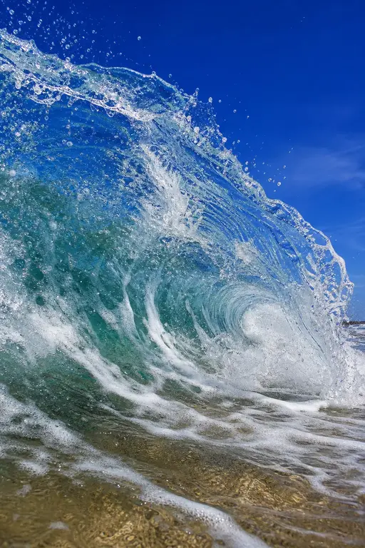
Real-time Breaking Waves for Shallow Water Simulations
1. Real-time Breaking Waves for Shallow Water Simulations
Nils Thürey1 Matthias Müller-Fischer2 Simon Schirm2 Markus Gross1
1ETH Zurich, Switzerland. thuereyn@inf.ethz.ch, grossm@inf.ethz.ch
2AGEIA Technologies, Switzerland. mmueller@ageia.com, sschirm@ageia.com
1.1. Abstract
We present a new method for enhancing shallow water simulations by the effect of overturning waves. While full 3D fluid simulations can capture the process of wave breaking, this is beyond the capabilities of a pure height field model. 3D simulations, however, are still too expensive for real-time applications, especially when large bodies of water need to be simulated. The extension we propose overcomes this problem and makes it possible to simulate scenes such as waves near a beach, and surf riding characters in real-time. In a first step, steep wave fronts in the height field are detected and marked by line segments. These segments then spawn sheets of fluid represented by connected particles. When the sheets impinge on the water surface, they are absorbed and result in the creation of particles representing drops and foam. To enable interesting applications, we furthermore present a two-way coupling of rigid bodies with the fluid simulation. The capabilities and efficiency of the method will be demonstrated with several scenes, which run in real-time on today's commodity hardware.
1.2. 1 Introduction
The field of fluid simulations has seen significant progress in the past years, particularly with respect to visual accuracy and application to various scenarios, such as interactions with different materials, phase changes and multi phase behavior. However, most of the advancements are not available for interactive environments, such as games. The major barrier is the extensive amount of computations necessary for solving a full 3D fluid motion, and tracing the free surface for rendering.
An effective way to increase the performance of the simulation of large bodies of liquids is the reduction of the problem from three to two dimensions. Instead of using 3D grid cells, the liquid is represented by a two dimensional height field. For calm situations, e.g., with smooth waves, this representation can still capture the main visual properties of the free surface fluid. Other situations, like overturn-
ing of waves at the shore line can, however, not be captured with such a reduced model. We propose a new technique to enhance efficient height field liquid simulation with particle based sheets, in order to create the effect of breaking waves. As a breaking wave is a highly turbulent process that is still not fully understood, we do not aim to fully simulate this phenomenon in real-time, but to capture its most important visual features.
Our approach consists of the following steps: the detection of potentially overturning wave regions, the generation of a fluid sheet to represent the wave, its advection and, finally, the coalescence with the 2D water surface. We represent the breaking wave with connected particles, which allows for the efficient and seamless creation of a surface mesh for rendering. In order to allow further interaction of the fluid with the environment, we apply two-way coupling of the shallow water simulation with rigid bodies. The capabilities of our method will be demonstrated with several test cases, from simple setups of single waves to more realistic environments such as breaking waves at a submerged shelf, or waves generated by rigid body interaction.
1.3. 2 Related Work
In the early years of fluid animation, procedural surface generation was used to represent breaking waves as described, e.g., by [6], [18] and more recently by [10]. For the simulation of open water surfaces, such as the ocean, spectral methods are often used, see [21], [8] and [14], among others.

Figure 1. Example of a game character surfing along a breaking wave in real-time.

Figure 2. Here an overview of our wave simulation approach can be seen.
Two-dimensional water simulations based on height fields offer more flexibility while keeping computational cost low. The capabilities of a simplified shallow water discretization for computer graphics were first presented in [11]. Furthermore, [17] extended a shallow water simulation with particle based splashes. [5] and [2] cover the basics of floating objects on the water surface. More recent work on shallow water simulations for real-time applications can be found in [12], where the authors apply noise textures for increased surface details, or [7] and [15], where wave simulations using the GPU are demonstrated.
Full 3D simulations became popular with the methods developed in [19] and [4], and have by now been extended in numerous ways. Studies of breaking waves have likewise first been performed in 2D [1]. [16] on the other hand presented a full 3D treatment of breaking waves with a Volume-of-Fluid simulation. In [20] the visual impact of breaking waves has been improved by adding particles for sprays and foam. Similar to [16], an approach to use slices of 2D simulations for wave simulations in real-time is demonstrated in [23]. Recently, Full three-dimensional simulations have been combined with two-dimensional techniques to speed up simulations of large volumes. In [9], a 2D simulation is performed beneath a layer of full 3D simulation for the fluid surface, while [22] couple the 3D simulation region to a 2D shallow water simulation. While these approaches significantly lower the simulation time, they are still not suitable for real-time applications.
Breaking waves have been simulated in the context of various computational fluid models. In the following we present a method for extending height field based simulations, such that the motion of breaking of waves can be computed. In particular, we will focus on shallow water simulations, as they yield a full velocity field for the fluid surface. In contrast to the spectral methods, they can, on the other hand, not handle the wave dispersion of deep water waves. It is, however, possible to apply our method to other simulation models that yield a height field and velocity vectors at the surface. Our simulation algorithm consists of the following steps: first, a normal shallow water sim-
ulation step is performed, as will be explained in the following section (3). Afterwards, the rigid body coupling of Section 7 is performed. In the next step the detection of overturning waves is handled (as will be explained in Section 4), and, finally, the advection of the generated particles is computed (Section 5).
1.4. 3 Shallow Water Simulations
The motivation to use shallow water (SW) simulations is to reduce the complex three dimensional description of a fluid to a simplified representation: a two dimensional height field. The corresponding equations are derived from the equations describing a full three dimensional fluid flow, the Navier-Stokes (NS) equations, by several simplifications. Note that, in the following, we will assume a gravity force along the axis, so the plane for the 2D wave simulations corresponds to the - plane. One simplifying assumption is that the velocity does not vary significantly along the axis, and that we have a constant pressure gradient from the water surface to the bottom. The only two forces driving the fluid are pressure and gravity. We furthermore make the assumption that we want to simulate liquids such as water, which effectively have a zero viscosity, and work with the simpler Euler equations. Thus, we can neglect the viscosity term of the NS equations.
To simplify the notation, will denote the partial derivative of the function along , where can be a spatial axis or time. In the following is the height of the water above ground, describes the bottom topography, and is the total height of water and terrain. The vector is the horizontal velocity of the fluid, and is the gravitational force perpendicular to the 2D simulation plane. The simulation region consists of grid nodes with size , and grid nodes with size in and direction, respectively. The simplified shallow water equations can now be written as
We use a staggered grid together with a semi-Lagrangian advection step [19] to solve these equations, as described by Layton et al. in [13]. As the height in a shallow water simulation is varying, and can be related to the pressure of a normal incompressible fluid solver, solving the SW equations does not require a pressure correction step, such as velocity projection. In comparison to solving only the wave equation for a water surface, a SW simulation, as described above, has the advantage of directly yielding a full velocity field for the surface. It can be used to, e.g., trace objects floating on the surface, and we will make use of it for coupling the SW and the rigid body simulations in Section 7. Moreover, SW simulations can be easily extended with a variety of boundary conditions, e.g., for flows through terrains, and can capture interesting effects, such as vortices behind obstacles in the flow.
1.5. 4 Wave Simulation
The following section will describe our approach to simulate breaking waves within the shallow water framework. We detect lines of steep wave fronts, and track these with a robust advection scheme. These wave lines generate patches of connected particles representing the fluid of an actual breaking wave. The wave lines adaptively track the original wave, and can merge with others in their neighborhood. An overview of our approach is shown in Figure 2.
Detection: Typically, a wave breaks when an initially smooth wave approaches a region of shallow water, e.g., a beach. The decreased height of the water causes the braking influence of the ground to become stronger. The wave steepens, and, at some point, overturns. Especially at beaches this effect is reinforced by the backward current of previous waves, causing a stronger difference between the forward movement of higher fluid layers, and the slower (or backward) movement of fluid layers near the ground.
The steepening of waves in regions of decreased fluid height can be reproduced with the shallow water equations. However, The effect of a breaking wave can naturally not be captured within a 2D simulation. The goal of the algorithm described in the following is to construct a line of connected points along each wave front that is a candidate for overturning. To actually detect the front of a steep wave, the gradient of the fluid height has to be larger than a given threshold . Moreover, the velocity of the fluid needs to be taken into account, otherwise not only the front, but also the back side of a wave will be detected. At the wave front the fluid velocity opposes the gradient of the height field. Hence, as a first step we identify a set of points in the shallow water grid, that fulfill the criterion:
Here, the gradient of the fluid height is computed with finite differences from the height field of the shallow wa-

Figure 3. Here a top view of the wave front region and line construction is shown.
ter simulation. The threshold is determined from the actual discretization of the shallow water equations, and a user defined parameter . The discretization influences the resulting shape of the waves by the gravitational force applied during each time step, while the parameter can be used to select the overall amount of waves to be generated. In the following we use , and compute as
The points of usually do not form a closed single layer along the wave front. To generate a sequence of connected points for along the wave front, we enlarge by adding all points that have a distance of less than to one of the points in . We have found that a distance of yields good results by closing gaps of this scale along the points fulfilling Equation (4). As multiple wave regions can be present at a single time step, this broadened set of points is segmented with a flood filling algorithm to identify disconnected regions. In the following, will denote such a single set of connected points of the broadened region. We select a random point from , and construct a line by following the tangent vector of the height field. On overview of this process is given in Figure 3.
This line construction is repeated for both tangent directions. With , these are given by and . The following procedure is first applied for one tangent direction, until the next point along this direction is not part of . Then the second part of the line is constructed along the opposing tangent direction. Given a point in , the next point is computed as
where denotes the current tangent direction. Due to the scaling of the tangent with , the line is constructed of points with a distance of the grid size of the simulation. To ensure the relatively large steps of Equation (6) do not by accident leave the region , the next point of is given by centering to the point of the steepest gradient as
Here the line consists of all points along the height field gradient at that are in . The point is added to and connected to . These steps are repeated until is not part of . In this case, the process of the line construction is restarted with the second tangent direction if , or the line is complete for . Likewise, if has a distance less than to the first point of the line, the line is completed by connecting the two points, resulting in a closed loop.
As the points in might also fulfill Equation (4) at a subsequent time step, all points of that are within a distance to an existing line are removed from the set. This prevents another line from being initialized right next to an existing one. Note that this approach does not deal with branches in the wave front region, but such a case will be handled by the construction of two lines, that might eventually merge (as explained below).
Advection: The wave speed for the shallow water equations is given by
However, for the interactive applications that we are targeting, the shallow water simulation can be distorted by a variety of factors, e.g., rigid bodies (as explained below) or other breaking waves. To accurately track the front of a shallow water wave with wave line , we combine an advection with the wave velocity, and a projection along the gradient direction onto the line of the steepest gradient on the wave front. The projection is performed with the bisection method, and an initial step size of length . Usually, 2-4 steps suffice to find the desired target point.
The direction of movement for a point of is given by the gradient of the height field from the last time step, at position . At this point in time was located at a correct position on the wave front, either from an initialization of the wave line, or from a previous advection step, and thus is used as the movement direction of at time .
As the wave crest might have passed , we first perform a projection along onto the maximum of the fluid height field. Once this maximum is found, we perform another forward projection onto the point of the steepest gradient on the wave slope at position . We now ensure that this new point is valid with respect to the original wave speed . If we remove the point from the line. Likewise, we ensure that this region of the wave is still steep enough to produce a wave. Thus, if , the point is also discarded.

Figure 4. This picture shows a side view of the wave line vertex advection.

Figure 5. Connection shapes for the mesh generation from refined and coarsened wave lines.
During its movement, the length of the wave front can change significantly. We thus adaptively resample the wave line by introducing new points when the distance between two neighbors is larger than . Similarly, points with a distance of less than are merged. A folding of the line can also be prevented by merging segments where holds. In both cases the new points are initialized by averaging the properties of the neighboring points. Hence, the resulting wave line consists of segments that have a similar scale as the grid size of the simulation throughout its lifetime.
1.6. 5 Wave Patch Generation:
The fluid sheet of an overturning wave is represented with a wave patch that is built from connected particles generated at the wave line. In time intervals a set of particles along the wave line is spawned for each point of the line, adding another layer of quads to the patch. Amongst each other, the particles have the same connectivity as the wave line. If a previous set of particles exists, the new set is connected to the previous one. If the same point on the line existed at the generation time of both particle sets, this is trivial. From these one-to-one connections, quads can be easily generated to form a closed surface of the wave patch. If points were added or removed from the wave line, these are marked, and corresponding connection shapes are inserted to guarantee a closed surface, as shown in Figure 5. To ensure that these three cases are sufficient, we only allow a single merging or insertion for a point within the time interval .
For the computation of the velocities of the wave patch particles, we use the velocity of the source point on the line . The actual overturning of a wave results in a significantly higher velocity at the top of the wave than at its bottom. We assume that this forward acceleration is proportional to the potential energy, in relation to the initial fluid height . Thus, the velocity of a wave sheet particle at position is given by
Here, is a parameter to control the strength of the height influence. As the wave line tracks the steepest point of the wave front, the generated particles have to be positioned at the wave crest to correctly give the impression of an overturning wave. The particle generation would be simplified if the crest of the wave was tracked instead of the front, as is done in our approach. However, the line of the wave crest is not as clearly defined, e.g., for saddle points and saddle lines of the height field. Thus, upon creation, the particles of the wave patch are moved to the crest along the inverted wave line velocity . We furthermore subtract from the particle position at the top of the wave, to ensure an overlap of the wave patch and the shallow water surface. This allows a smooth transition from the height field values to the wave mesh, as explained below in more detail.
Once the fluid represented by the wave patch is detached from the fluid below that represented by the shallow water simulation, its motion is primarily determined by its initial velocity and gravity. Thus, Euler steps are sufficient to integrate velocity and position over time. After the update, we perform a collision detection of the particle with the fluid surface of the shallow water simulation. When a collision is detected, we distort the shallow water simulation at the particle position with , while the eight neighbors of the shallow water node at are displaced by . Note that we do not explicitly transport fluid with the wave patches, as a modification of the height field along the wave front would distort its motion. This leads to noise within the shallow water simulation, unless the modification along the whole region of the wave is very smooth. As mentioned below, correctly performing this mass transport and smoothing is a topic of future research.
| Task | Duration |
|---|---|
| Shallow water simulation | 39.6 % |
| Breaking waves & particle simulation | 21.7 % |
| Mesh generation (vertices & normals) | 18.9 % |
| Rendering & graphics engine | 19.8 % |
Table 1. Computational requirements of the different parts of our algorithm.
| Test case | Resolution | Frames per Second |
|---|---|---|
| Single waves | 43.6 | |
| Box interaction | 51.8 | |
| Submerged shelf | 75.2 | |
| Surfer | 40.6 |
Table 2. Frames per second measurements for the different test cases.
1.7. 6 Rendering the Waves
For the rendering of a wave patch, its particles with their connectivity can be directly reused as vertices. The wave patches already represent a close surface, which, however, does not have a thickness. Thus, we create two instances of this surface for rendering, and displace the second one downward along the normal direction. To get a closed mesh, the sides of these two meshes are connected with quads. As mentioned above, the initial position of the particles of the wave patch ensures an overlap with the shallow water surface. It correctly represents the top of the wave, while the displacement of the lower side is chosen to represent the mass of the fluid according to the parameter . Given a particle on the wave patch that is used as a vertex for the upper mesh, the position of the corresponding second vertex is given by .
By observing real breaking waves it can be seen that a wave does not break as a whole at once, but the breaking process starts at a given position. It then spreads outward along the wave front due to the viscosity of the water. To achieve this effect, we select a the mid point of the wave line as the tip of the breaking wave. The wave patches are then generated from an enlarging region centered around the initial point. This is visible in, e.g., Figure 6.
In contrast to full 3D simulations, it is furthermore easy to generate texture coordinates for the fluid surface of the wave patch. For a point on the wave line , its texture coordinate is given by its lifetime, and its position in the line. We, e.g., use these texture coordinates to blend in a foam texture at the tip of the wave patch.
Finally, to give the impression of a larger scale, we use standard particles. These are generated when the particles of the wave patch hit the shallow water surface. Moreover, particles are spawned along the tip of the wave patch. Here, in reality, the drag of the air causes disturbances of the fluid sheet, resulting in the formation of drops. For the pictures shown in this paper, we furthermore use a small scale bump map to distort the reflective shallow water surface, which gives the impression of smaller surface waves.

Figure 6. Different types of waves created by our method.
1.8. 7 Two-Way Rigid Body Coupling
A straight forward approach for simulating the interaction of rigid bodies with the water surface is to have each body push down the water columns beneath it in order to remove all overlaps. To conserve the water volume, the volume that is added or removed from each column has to be compensated for in other parts of the domain. This method yields nice waves for bodies dragged through the water. The major drawback of the approach, however, is the fact that it cannot handle the situation when a body is pulled beneath the surface and gets fully submerged. In that case, the water does not collapse above it leaving a hole of the size of the body in the surface.
The method we propose here is similar but solves the problem of submerged bodies. In addition to the height value we store a value at each cell, which represents the water volume that is displaced by one or more rigid bodies. This value does not influence the simulation directly. At the beginning of a time step the area of each body is projected onto the - plane. For each cell at position that is covered by the projection we compute the new value as the length along the column at that is covered by

Figure 8. A user interacts with several boxes that were thrown into a simulated basin.
rigid bodies. The difference indicates the change in volume covered by bodies between the current and the last time step. This change is distributed to the four direct neighbor cells, similar to algorithms for changing ground depth. Hence, for a grid cell at position with a neighbor cell at
The positions of the four neighboring cells are given by and , respectively. This way, the water surface closes nicely above the body. The scheme conserves volume even for . By changing the amplitudes of waves generated by bodies can be adjusted. Pulling bodies down or out of the water results in plausible increase and decrease of the water level. The value of can be positive or negative and give rise to both, the bow wave in front and the wake at the back of a body that is dragged through the water.
For a coupling in the other direction, we add a force of the water displacement and fluid velocity for each of the grid nodes at position covered by the rigid body:
where is a constant to set the density of the fluid. Integrating these forces over the region of the rigid body and over time, will cause the rigid body to float or sink depending on its mass, and swim along with the fluid velocities.
1.9. 8 Results
The capabilities of our wave simulation approach are demonstrated with the test cases shown in Figure 6. Each of the three rows of pictures show a breaking wave generated from an initial pulse, which has a height of in comparison to the overall height . The breaking wave of the upper row of Figure 6 was generated with a box profile aligned with the grid boundary. The wave front is correctly detected and tracked throughout its motion. To demonstrate that our method works regardless of the alignment of the wave, the middle row uses an initial height profile that is rotated by ten degrees. The lower row of pictures was generated with a square elevation initialized in the middle of the simulation grid. This results in a circular wave that spreads outward. Note that the sharp edge of these three profiles results in the detection of several smaller waves in the region behind the main wave front. They are, however, quickly removed from the simulation once the steepness criterion of Equation (4) is not met anymore.

Figure 7. A smooth wave approaches a submerged shelf, which results in a steepening of the wave and, eventually, overturning. The ground topography is visible below the shallow water surface.
Images from one of our test simulations with rigid body interaction can be seen in Figure 8. Several boxes are thrown into a basin of fluid, become submerged, are dragged along with the fluid, or float on the surface. A user can interact with the simulation by moving around the boxes. The simulation remains stable even during quick movements.
A simulation of a breaking wave at a submerged shelf is shown in Figure 7. Test cases with a submerged shelf are common in coastal engineering, and represent the typical topology of a shore area. A simulation of a breaking wave at a submerged shelf in 3D was demonstrated in, e.g., [3]. With our algorithm we can recreate this phenomenon in real-time. Here, an initially smooth wave, that would not break on even ground, is approaching the submerged shelf. The decreasing fluid height causes the wave to steepen within the shallow water framework. Eventually, the wave is steep enough to fulfill Equation (4), and triggers the creation of a breaking wave. Note that the shelf is not fully aligned with the simulation grid, which causes the wave to start breaking further towards the viewer.
Finally, we have recreated a game scene of a surfing character in Figure 9. Our algorithm yields sufficient detail even when the camera is very close to the breaking wave. The details of the breaking wave can be controlled by changing the point distances on the wave line, as this also results in a change of the mesh resolution.
A limitation of our approach is that it doesn't properly handle cases with chaotic waves in the shallow water simulation. This causes the detected breaking waves to be removed before they can fully develop. Thus, the algorithm is not suitable for handling situations that would require many small splashes or drops, but targeted towards larger entities like a whole wave. Likewise, small scale waves caused by
moving objects, can only be simulated with breaking if they are properly represented within the shallow water simulation.
The results discussed in this section were calculated on a common PC with an Intel Core 2 Duo CPU (2.13 GHz), and a Nvidia Geforce 7950 GPU. As our implementation is not yet parallelized, it only makes use of one of the cores of the CPU. The actual frame rates of the different cases are given in Table 2. All test cases use between 160k and 200k grid points, and run with 40 to 75 frames per second, including rendering. The distribution of the computational time for the different parts of our algorithm can be found in Table 1. For this measurement a typical wave, as shown in Figure 6, was simulated. Overall, the fluid simulation amounts for 80% of the run time, while the rendering and overhead introduced by the graphics engine require the remaining 20%. Roughly half of the simulation time is spent on the shallow water simulation itself, while the wave simulation algorithm requires circa one fourth of the time. The creation of the surface mesh and the computation of the normals again requires roughly one fourth of the computations.
1.10. 9 Conclusions
We have presented a new method to perform real-time simulations of open water scenes with breaking waves. It is based on detecting and tracking the wave front with line segments. The breaking wave itself is represented by a patch of connected particles. Our model for coupling a rigid body simulation with the shallow water simulation moreover makes it possible to create interesting interactive applications, and can handle cases such as submerged bodies. Overall, the algorithm performs with high frame rates, and without causing noticeable slowdowns during the course of the simulation. It furthermore allows the efficient and seamless creation of a textured surface mesh. These properties of the algorithm make it especially interesting and suitable to be used in computer games. Although it is aimed for real-time applications, the algorithm is also interesting for high quality off-line animations. It could, e.g., allow the efficient simulation of large open water shore scenes, while giving animators real-time feedback during their work.

Figure 9. A scripted character is moved along the wave front, giving the impression of surf riding.
In the future we would like to extend our algorithm by, e.g., detecting collisions between different wave patches, and performing a full smoothed particle hydrodynamics simulation of the splash and foam particles. This would allow the correct handling of more chaotic or quickly changing scenes. The plausibility of the simulations could also be increased by a model for transporting fluid volumes from the shallow water simulation with the breaking wave and particles. Furthermore, it would be interesting to combine our technique with an adaptive algorithm to create detailed triangulations of the fluid surface and the drops. This would be especially interesting for the off-line simulations mentioned above.
1.11. 10 Acknowledgements
We thank AGEIA for funding this research project.
1.12. References
- [1] G. Chen, C. Kharif, and S. Zaleski. Two-dimensional navier-stokes simulation of breaking waves, 1999.
- [2] J. X. Chen, N. da Vitoria Lobo, C. E. Hughes, and J. M. Moshell. Real-time fluid simulation in a dynamic virtual environment, 1997.
- [3] D. Enright, S. Marschner, and R. Fedkiw. Animation and Rendering of Complex Water Surfaces. ACM Trans. Graph., 21(3):736–744, 2002.
- [4] N. Foster and R. Fedkiw. Practical animation of liquids. In Proc. of ACM SIGGRAPH, pages 23–30, 2001.
- [5] N. Foster and D. Metaxas. Realistic Animation of Liquids. Graphical Models and Image Processing, 58, 1996.
- [6] A. Fournier and W. T. Reeves. A simple model of ocean waves. In SIGGRAPH '86: Proceedings of the 13th annual conference on Computer graphics and interactive techniques, pages 75–84, New York, NY, USA, 1986. ACM Press.
- [7] T. R. Hagen, J. M. Hjelmervik, K.-A. Lie, J. R. Natvig, and M. O. Henriksen. Visual simulation of shallow-water waves. Simulation Modelling Practice and Theory, 13, 2005.
- [8] D. Hinsinger, F. Neyret, and M.-P. Cani. Interactive Animation of Ocean Waves. July 2002.
- [9] G. Irving, E. Guendelman, F. Losasso, and R. Fedkiw. Efficient Simulation of Large Bodies of Water by Coupling Two and Three Dimensional Techniques. ACM Trans. Graph., 25, 2006.
- [10] S. Jeschke, H. Birkholz, and H. Schmann. A procedural model for interactive animation of breaking ocean waves, 2003.
- [11] M. Kass and G. Miller. Rapid, Stable Fluid Dynamics for Computer Graphics. ACM Trans. Graph., 24(4):49–55, 1990.
- [12] T. Klein, M. Eisele, D. Weiskopf, and T. Ertl. Simulation, modelling and rendering of incompressible fluids in real time, 2003.
- [13] A. T. Layton and M. van der Panne. A Numerically Efficient and Stable Algorithm for Animating Water Waves. The Visual Computer, 18/1:41–53, 2002.
- [14] J. Lovisnach. Complex Water Effects at Interactive Frame Rates. Journal of WSCG, 11:298–305, 2003.
- [15] M. M. Maes, T. Fujimoto, and N. Chiba. Efficient animation of water flow on irregular terrains. In GRAPHITE, pages 107–115, 2006.
- [16] V. Mihalef, D. Metaxas, and M. Sussman. Animation and Control of Breaking Waves. Proc. of the ACM SIGGRAPH/Eurographics Symposium on Computer Animation, pages 315–324, 2004.
- [17] J. F. O'Brien and J. K. Hodgins. Dynamic simulation of splashing fluids. In CA '95: Proceedings of the Computer Animation, page 198, 1995.
- [18] D. R. Peachey. Modeling waves and surf. In SIGGRAPH '86: Proceedings of the 13th annual conference on Computer graphics and interactive techniques, pages 65–74, New York, NY, USA, 1986. ACM Press.
- [19] J. Stam. Stable Fluids. Proc. of ACM SIGGRAPH, pages 121–128, 1999.
- [20] T. Takahashi, H. Fujii, A. Kunitatsu, K. Hiwada, T. Saito, K. Tanaka, and H. Ueki. Realistic animation of fluid with splash and foam. Computer Graphics Forum, 22 (3), 2003.
- [21] J. Tessendorf. Simulating Ocean Surfaces. SIGGRAPH 2004 Course Notes 31, 2004.
- [22] N. Thürey, U. Rüdte, and M. Stamminger. Animation of Open Water Phenomena with coupled Shallow Water and Free Surface Simulations. Proc. of the ACM SIGGRAPH/Eurographics Symposium on Computer Animation, 2006.
- [23] Q. Wang, Y. Zheng, C. Chen, T. Fujimoto, and N. Chiba. Efficient rendering of breaking waves using mps method, Jun 2006.