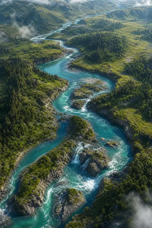
Procedural Riverscapes

1. Procedural Riverscapes

A. Peytavie¹, T. Dupont¹, E. Guérin¹, Y. Cortial¹, B. Benes², J. Gain³, and E. Galin¹

¹CNRS, Université de Lyon, LIRIS, France ²Purdue University, USA ³University of Cape Town, South Africa

1.1. Abstract

This paper addresses the problem of creating animated riverscapes through a novel procedural framework that generates the inscribing geometry of a river network and then synthesizes matching real-time water movement animation. Our approach takes bare-earth heightfields as input, derives hydrologically-inspired river network trajectories, carves riverbeds into the terrain, and then automatically generates a corresponding blend-flow tree for the water surface. Characteristics, such as the riverbed width, depth and shape, as well as elevation and flow of the fluid surface, are procedurally derived from the terrain and river type. The riverbed is inscribed by combining compactly supported elevation modifiers over the river course. Subsequently, the water surface is defined as a time-varying continuous function encoded as a blend-flow tree with leaves that are parameterized procedural flow primitives and internal nodes that are blend operators. While river generation is fully automated, we also incorporate intuitive interactive editing of both river trajectories and individual riverbed and flow primitives. The resulting framework enables the generation of a wide range of river forms, ranging from slow meandering rivers to rapids with churning water, including surface effects, such as foam and leaves carried downstream.

1.2. 1. Introduction

Authoring realistic virtual landscapes is a perennial challenge in computer graphics. It involves modeling the entirety of a natural scene including terrain, vegetation, cities or villages, road networks, cloudscape, watercourses, and their interdependence. The results have broad application to computer-generated movies, games, and virtual environments. While there has been significant progress in capturing individual phenomena, the dynamic aspects of landscapes have been relatively under-explored. This is unfortunate, because dynamic effects, such as wind and water flow, where present, have strong visual saliency.

There is a large body of previous work that focuses separately on terrain modeling and fluid simulation. However, the combined modeling of riverbeds and water surface animation has not received concomitant attention. The challenge stems not only from the complex structure of riverbeds, ranging from meandering courses to braided sub-channels, but is also due to the complexity of local water movement. Our central strategy is to rely on archetypes for building riverbed geometry and water surface behaviour. Importantly, this circumvents the need for computationally demanding fluid simulation and allows a unified procedural approach.

Specifically, from the starting point of a bare-earth terrain, either sourced from existing digital elevation models, generated procedurally, or modeled by the user, and with a range of permissible sampling resolutions (1m - 30m per pixel), a plausible river network is derived according to the Rosgen classification used in hydrology, inscribed into the terrain, and populated with a consistent animated water surface. The resulting river structure and dynamics can also

be interactively edited by the user, who can position and adjust the procedural elements of the scene.

In more detail, we take as input a digital elevation model, evaluate its hydrological characteristics, and specify the course of a detailed, possibly branching river network (see Figure 1). Detailed riverbed cross-sections are then derived using Rosgen classification and flow characteristics and the resulting geometry can be inscribed into the terrain heightfield. Then an attendant blend-flow tree is generated automatically. For instance, cascade primitives are placed after step-wise drops in elevation, while basins will be populated with calm water primitives. Our key observation is that visually a river surface is in a steady flow state, and displays only small periodic, and random perturbations. For example, the unperturbed wake behind a submerged rock varies subtly in form, but not in position. Movement is also predominantly in $2\frac{1}{2}D$ , with the occurrence of locally significant patterns such as vortices, ripples, whirlpools, and small cascades. Rather than implementing a full fluid simulation with the attendant scaling issues, we blend animated procedural primitives to capture these cyclical patterns.

Our technical contributions include: 1) a procedural pipeline for generating extensive, complex, branching rivers courses on bare-earth terrains, 2) the adapted carving of a riverbed according to the Rosgen classification scheme, 3) a novel blend-flow tree representation, which provides a function-based composite water surface that can be animated in real-time, 4) user control over the procedural scene elements, which allows effective authoring of riverscapes.

Figure 1: A workflow diagram showing the process from a bare-earth input terrain to a detailed river course. The workflow includes: Terrain (raw data), Network (graph), Slope (calculated), and Drainage (calculated). These are combined into a 'Bare-earth terrain' visualization, which is then processed into 'Terrain with river' showing the final river course.

Figure 1: From a bare-earth input terrain, our method calculates the slope and drainage area to automatically generate a river graph that is procedurally amplified into a detailed river course. In this case, 4.266km-long, with 63k terrain and 42k flow primitives.

1.3. 2. Related Work

Our paper addresses the problem of user-controlled large-scale procedural river modeling and animation. We thus relate our work to riverbed modeling and river animation. For a more general perspective we refer the reader to works on fluid simulation [Bri15], terrain modeling [GGP*19], and general procedural methods [EMP*02].

State-of-the-art methods have focused in isolation on fluid animation, coarse river networks, or modeling terrains without rivers. No current method produces a coherent combination of a hydrologically-defined bedded river network and corresponding river animation.

1.3.1. 2.1. Riverbed Generation

River modeling can be categorised based on spatial range into river network, valley, and riverbed modeling.

River networks: Consideration of the interaction of rivers and terrain has a long history in computer graphics: Kelley et al. [KMN88] were the first to procedurally generate river networks, followed soon afterwards by Prusinkiewicz and Hamel [PH93] who combined L-systems with terrain erosion. Derzapf et al. [DGGK11] produce procedural river networks on a planetary scale and Gnevaux et al. [GGG*13] use a procedural approach inspired by geology and hydrology to generate terrains with embedded medium-scale rivers. Creating valleys on an existing map can be performed using hydraulic erosion algorithms [BTHB06, KBKS09], accelerated by GPU implementation [MDH07, SBBK08]. This carves valleys at coarse scales, but does not handle the finer definition of riverbeds. The few methods that address riverbed carving either rely heavily on manual editing and sketch-based interfaces [BN08, EPCV15, HGA*10] or do not address fine-scale detail [GGP*15].

Our approach differs in that we focus on structurally analyzing existing terrains to identify and carve river courses rather than addressing the wholesale modeling of terrains [GGG*13, GGP*15]. As a part of this structural analysis, we use Rosgen templates [Ros94] and Horton Strahler numbering [Hor45], which are common and crucial models in geomorphology. Contrary to Gnevaux et al. [GGG*13], we explicitly employ the river profiles and paths as parameters for procedurally sculpting riverbeds. Crucially, our riverbed carving is compatible with the generation of an

animated river surface, which is beyond the purview of previous terrain methods.

1.3.2. 2.2. Water Animation

When dealing with rivers, water animation is highly constrained by the profile and trajectory of the river. This observation is particularly relevant for simulation methods but also applies to procedural animation.

Simulation: Theoretically, any simulation method could be used in the context of watercourse animation. However, in typical cases, a river can extend up to several kilometers, presenting a significant challenge in the trade-off between precision, simulation time and memory overhead. Some methods bypass this by directly optimizing the simulation process [LvdP02, LH10, KW06, IGLF06, NB11]. Another possibility is to enhance detail using wavelets to represent turbulence [KTJG08] or specialized particles [HW04, CM10, TMFG07]. A third tack is to enhance particles to carry supplementary information, thereby simplifying simulation [SRF05, YHK07, JW17, JSMF*18]. In a sense, these particles are a step towards our animated riverflow primitives. The main limitation of simulation is a lack of control, particularly when it comes to predicting and controlling how particles behave at the boundary of the riverbed. Notably, several simulation methods are simply not adapted to the continuous flowing of water from a spring to a sink and only deal with flat water bodies such as lakes.

Procedural methods: In contrast, procedural techniques manage to overcome these limitations and define the animation of water using phenomenological methods. This extends to the procedural representation of animated rivers. Neyret et al. [NP01], and later improvements [YNBH09, YNS11], focus on the procedural animation of quasi-stationary waves and ripples in brooks and small streams. It is worth noting that our method adopts a similar strategy, but is more general in application. Cheney [Che04] introduces Flow Tiles, which are bounded divergence-free velocity field patches that can be used to tile an animated domain, such as cloudscapes, riverscapes, and grasslands. The tiles serve a similar role to our primitives, but are limited in their placement and combination. Stomakhin et al. [SS17] control fluid-based animations by introducing Flux Animated Boundary primitives with a view to guiding physically-based particle simulations. Nugjar et al. [NC13] simulate a river with smoothed particle hydrodynamics, and then derive a Markov field, which is replayed afterwards.

Figure 2: Method overview diagram. The process starts with 'Terrain T' (a 2D heightfield). This leads to 'Analysis', which produces 'Rosgen types' (A, B, C) and a 'Graph G'. These are used in 'Amplification' to create 'Primitives' (Water primitives P and Riverbed primitives R). These are then combined in 'Combination' to form a 'Layered model' (Animated water f(p, t) and Riverbed function h(p)). Finally, 'Rendering' produces 'Final images'.

Figure 2: Method overview: the input is a 2D heightfield from which flow characteristics are automatically derived. A river network and riverbed geometry are constructed using Rosgen categorization (see Figure 3). Next, derived slope, water volume, and flow velocity values for each map cell in the river are fed to a procedural amplification process. The output is a river model in the form of a blend-flow tree that encodes a temporal water elevation function $f(\mathbf{p}, t)$ , which can be rendered in real time or off-line.

Previous work has shown significant progress in the generation of either detailed water movement or hydraulically-carved terrain. However, to our knowledge, ours is the first procedural method that guarantees an animation that is coherent with the riverbed relief. This is achieved by consistently carving riverbeds into existing terrains and producing the associated water surface animation.

1.4. 3. Workflow

Our procedural amplification framework, supplied with a terrain as input, provides a landscape with an animated river system, consisting of riverbed geometry coupled with an animated water surface, as output.

The workflow is outlined in Figure 2; it begins with a user-supplied heightfield, obtained, for example, as a scanned digital elevation model or generated by a terrain modeling system. Overlay maps for slope, drainage area, and stream power are derived as a first step.

Our work uses the Rosgen river classification [Ros94] that defines the detailed characteristics of the geometry of the riverbed (i.e. the cross section and longitudinal profile, sinuosity, riverbed materials, entrenchment ratio) according to the local slope and flow of the river. From this combined terrain data we generate a river network graph, whose edges correspond to river segments labeled by Rosgen type (see Figure 3). This results in a parameterized river network with per-cell waterflow values for slope, volume, and velocity. From this information the shape of the riverbed can be derived and inscribed into the terrain.

Next, the river network is refined, based on this flow data and the geometry of the riverbed, by appropriately placing localized animated primitives that represent cycling water patterns, such as waves, whirlpools, and cascades. Overlapping primitives are combined using blend operators into a hierarchical blend-flow tree that defines the animated surface of the water as a function $f(\mathbf{p}, t)$ . This procedural function can be directly evaluated at any point and time without the need for simulation. Finally, the combined procedural river representation can be rendered directly at real-time rates or passed on to an off-line process to generate photo-realistic images.

Figure 3: Overview of different Rosgen river types (A, B, C or D). The figure shows four panels (A, B, C, D) illustrating different river types. Each panel includes a 'Refined Trajectory E' (longitudinal profile) and a 'Cross section' (orthogonal cross-section).

Figure 3: An overview of different Rosgen river types (A, B, C or D), along with their characteristic detailed trajectory templates $\tilde{E}$ . The classification is based on both the orthogonal cross-section and longitudinal trajectory of rivers found in nature.

The initial automated placement of procedural primitives may not always match an animators intent and so our framework supports editing at various levels of abstraction: individual primitives can be inserted, removed or fine-tuned; the river graph can be edited; and, if necessary, the terrain can be locally remodeled and the river network regenerated.

1.5. 4. River Network Graph

In many cases a river graph, with the attendant parameters required for river network amplification, is not available for a given input terrain. Rather than expect a user to undertake a laborious markup process, we instead provide a procedural river network analysis step (see Figure 4) that works off a simple bare-earth terrain represented as Digital Elevation Model (DEM).

The analysis proceeds as follows: given a terrain $\mathcal{T}$ composed of regular grid cells $C_{ij}$ , we first generate a discretized river network $\mathcal{D}$ , and then convert it into a river network graph $\mathcal{G}$ with nodes and edges labelled with flow data, as a precursor to river network amplification (as described in Section 5).

We begin by computing the drainage area $A_{ij}$ for every cell $C_{ij}$ of the input terrain $\mathcal{T}$ (using the method of Freeman [Fre91]). The discrete river network $\mathcal{D}$ is then simply the set of cells that have a drainage area greater than a user-controlled threshold value (see

$Figure 4: Overview of river network derivation. The process starts with a 'Terrain \tau' which is used to create a 'Drainage Area \mathcal{A}'. This leads to a 'Discrete network \mathcal{D}' represented as a grid of cells. From the discrete network, 'Graph creation' produces a 'Continuous River Graph \mathcal{G}'. The graph consists of nodes \mathcal{N}_i and edges \mathcal{E}(t_{ik}), where each edge is associated with a Rosgen type \mathcal{N}_k(\phi_k, s_k).$

Figure 4: Overview of river network derivation. The process starts with a 'Terrain \tau' which is used to create a 'Drainage Area \mathcal{A}'. This leads to a 'Discrete network \mathcal{D}' represented as a grid of cells. From the discrete network, 'Graph creation' produces a 'Continuous River Graph \mathcal{G}'. The graph consists of nodes \mathcal{N}_i and edges \mathcal{E}(t_{ik}), where each edge is associated with a Rosgen type \mathcal{N}_k(\phi_k, s_k).

Figure 4: An overview of river network derivation: We first extract maps from the terrain and calculate the discretized network $\mathcal{D}$ . This is then converted to a graph $\mathcal{G}$ , with flow $\phi_k$ and slope $s_k$ data for every node $\mathcal{N}_k$ and a Rosgen type $t_{ik}$ for edges $\mathcal{E}_{ik}$ .

Figure 5). One complication is that the drainage calculation assumes that there are no depressions (local minima) in the digital elevation model, since these have no outlet to neighboring cells. To prevent disconnected river graphs we apply an optimal depression filling algorithm [BLM14], which leaves the surface slightly proud with an available flow channel.

$Figure 5: Four maps showing parameters characterizing different parts of the river network. From left to right: 'River Network \mathcal{G}' (a network of blue lines on a brown terrain), 'Drainage \mathcal{A}' (a map showing blue drainage areas), 'Stream Power \mathcal{P}' (a map showing blue stream power values), and 'Slope S' (a map showing blue slope values).$

Figure 5: Four maps showing parameters characterizing different parts of the river network. From left to right: 'River Network \mathcal{G}' (a network of blue lines on a brown terrain), 'Drainage \mathcal{A}' (a map showing blue drainage areas), 'Stream Power \mathcal{P}' (a map showing blue stream power values), and 'Slope S' (a map showing blue slope values).

Figure 5: Parameters characterizing different parts of the river network: the slope $S$ and stream power $\mathcal{P}$ relate to erosive forces, while the drainage area $\mathcal{A}$ dictates the flow volume.

The discrete river network is then converted into a continuous graph $\mathcal{G}$ by defining a node at cells with more than one contributor and smoothing the trajectory of the river between nodes with piecewise cubic splines.

Next, graph nodes are labeled with the terrain slope $s$ and river flow $\phi$ values at their cell position. The latter is a measure of the volumetric rate at which water is carried down the river and an accurate estimation is problematic, since it depends on parameters such as rainfall and soil composition. Instead, we apply a simplified model based on an empirical power law observed in geomorphology [Dun78]: from drainage area $A_{ij}$ [ $m^2$ ], the flow $\phi_{ij}$ of the river [ $m^3 s^{-1}$ ] is approximated by $\phi_{ij} = 0.42A_{ij}^{0.69}$ . This equation takes into account evaporation and infiltration, which is why the volume of flow is not preserved.

The labeling of graph edges is more involved, since classification by Rosgen type [Ros94] requires a computation of the following river properties: segment-based river flow, stream power, and the Horton-Strahler number. First, river flow $\phi_{ij}$ is averaged over the cells occupied by the edge. Then, the stream power, which captures the erosive action of water flowing in the river [CBC*16], is calculated based on slope $S_{ij}$ and drainage area $A_{ij}$ per edge cell as:

$P_{ij} = A_{ij}^{1/2} \cdot S_{ij}$ , and averaged. The final derivation is of the Horton-Strahler number [Hor45], a numerical measure of branching complexity, with higher numbered river segments having more feeder tributaries. With this the river network graph is fully labeled and can be passed directly to the River Network Amplification process described in Section 5.

1.6. 5. River Network Amplification

Provided with a river network in the form of a graph $\mathcal{G}$ (see Section 4), we automatically generate a detailed trajectory for the river course, carve the corresponding riverbed into the terrain surface, and seed riverflow primitives from which a blend-flow tree is constructed to animate the river surface (see Figure 6). Collectively, this constitutes a procedural amplification of the riverscape.

$Figure 6: Diagram of the procedural amplification process. It starts with a 'River edge \mathcal{E}_{ij}' which undergoes 'Rosgen analysis' and 'Trajectory refinement' to produce a refined trajectory \tilde{\mathcal{E}}_{ij}. This is then used for 'Riverbed and water generation' to create 'Riverbed primitives \{\mathcal{R}_k\}'. The process also involves 'Water primitives \{\mathcal{Q}_k\}' and 'Riverbed primitives \{\mathcal{R}_k\}' which are used to generate 'Rivered primitives \{\mathcal{P}_k\}'.$

Figure 6: Diagram of the procedural amplification process. It starts with a 'River edge \mathcal{E}_{ij}' which undergoes 'Rosgen analysis' and 'Trajectory refinement' to produce a refined trajectory \tilde{\mathcal{E}}_{ij}. This is then used for 'Riverbed and water generation' to create 'Riverbed primitives \{\mathcal{R}_k\}'. The process also involves 'Water primitives \{\mathcal{Q}_k\}' and 'Riverbed primitives \{\mathcal{R}_k\}' which are used to generate 'Rivered primitives \{\mathcal{P}_k\}'.

Figure 6: Our procedural amplification takes a coarse river trajectory $\mathcal{E}$ and refines it according to the Rosgen type. Riverbed primitives $\mathcal{R}$ for geometry carving and riverflow primitives $\mathcal{P}$ for water animation are then seeded over the river domain.

The river graph $\mathcal{G}$ has nodes $\mathcal{N}_i$ that correspond to river junctions and edges $\mathcal{E}_{ij}$ that represent the intervening trajectory of the river. The graph nodes store geomorphological data; in particular, the average slope $s_i$ in the local neighborhood of the node and the flow of the river $\phi_i$ . Graph edges, meanwhile, store their Rosgen type $t_{ij}$ (see Figure 3) and encode the river trajectory as a piecewise-cubic curve.

Amplification proceeds by first refining the trajectories of edges $\mathcal{E}$ in the river graph $\mathcal{G}$ , based on their Rosgen type (see Section 5.1). The result is a revised geometric graph $\hat{\mathcal{G}} = \{\mathcal{N}, \hat{\mathcal{E}}\}$ . Importantly, this process not only adjusts the planar $(x, y)$ course of the river, but also its longitudinal profile ( $z$ elevation values along the river spine) so as to create appropriate basins, pools and cascades. Then, the geometry of the riverbed is realised, by selecting, scaling and assigning Rosgen cross-sectional templates along the river, and carved into the terrain $\mathcal{T}$ , which results in a modified terrain $\hat{\mathcal{T}}$ (Section 5.2). Finally, we distribute riverflow primitives (Section 5.3), in readiness for their assembly into a blend-flow tree that defines the animated water surface.

1.6.1. 5.1. Analysis and Trajectory Refinement

For every river segment $\mathcal{E}_i$ in $\mathcal{G}$ , we generate a refined three-dimensional trajectory $\tilde{\mathcal{E}}_i$ , depending on its computed Rosgen type $t_i$ . The horizontal trajectory can be meandering if the local slope $s_i$ is low and the flow $\phi_i$ moderate (type C, E or G), or straight if the slope is steep (type A or A+). Afterwards, the longitudinal elevation profile of the trajectory is also refined with a view to creating drops and basins keyed to the Rosgen type (see Figure 7 and 9). This is important since the riverbed slope is one determinant of cascade, wave and turbulence placement.

Figure 7: The longitudinal profile of a river. The left diagram shows a 'Low resolution terrain T' with a 'Low resolution water depth' profile. The right diagram shows a 'Carved riverbed h(p)' with 'Calm' water, a 'Waterfall', 'Turbulent' water, a 'Basin', and a 'Cliff'. Above the right diagram is the text 'Animated water f(p, t)'.

Figure 7: The longitudinal profile of a river is refined by 1) randomly sampling the river trajectory and 2) flattening the water level and riverbed between certain samples based on Rosgen type, and subsequently instantiating procedural primitives based in part on the revised profile.

Figure 8: Scaling of template cross sections. The diagram shows a cross-section C(t) with a velocity profile u. The area a is defined as a = phi / ||u||.

Figure 8: Scaling of template cross sections.

We check that the river height is monotonically decreasing. When this fails, we propagate the heights of the river trajectories downwards and perform local adjustments at the junctions. If the riverbed slope is greater than a threshold, we adjust the height by inserting cascades and leveling the profile.

Rosgen templates also define cross-sections $C(r)$ taken orthogonal to the river direction and of unit area (Figure 8). Therefore, we need to calculate the river area from the flow in order to scale the template. Therefore, for every template cross section $C(r)$ , the scaling factor is defined as the area $a = \phi / \|u\|$ with $\phi = 0.42A^{0.69}$ (see Section 4).

Figure 9: The influence of slope. The left image shows 'Rosgen A+' with a steep river (s = 6%) featuring drops and basins. The right image shows 'Rosgen B' with a flatter river (s = 0.1%) featuring calm water and ripples.

Figure 9: The influence of slope: [Left] a steep river ( $s = 6\%$ ) of Rosgen type A+, which gives rise to drops and basins, and matching cascades and turbulence; [Right] a flatter river ( $s = 0.1\%$ ) with the same planar trajectory, which results in calm water primitives with a few ripples.

1.6.2. 5.2. Riverbed Carving

From the refined river trajectory and its Rosgen type, riverbed geometry $\mathcal{R}$ can be constructed and embedded in the terrain (Figure 10). For this we employ normalized cross-sectional and longitudinal Rosgen templates. These are inspired by the cross sections

$C(r)$ in Figure 3, but also depend on the local curvature of the river trajectory. They are normalized in the sense that their scale assumes unit area for water in the cross section, and when instantiated, they are scaled according to a factor derived from the flow $\phi$ and elevation of the trajectory.

Figure 10: Terrain tree representation of the riverbed R of Rosgen type A with cascade and basin. The diagram shows a tree structure with nodes: 'Replace' (connected to 'Merge' and 'Terrain'), 'Merge' (connected to 'Merge' and 'Basin'), 'Merge' (connected to 'Merge' and 'Flat'), 'Basin', 'Flat', 'Cascade', and 'Riverbed'. To the right is a 3D model of a riverbed with a 'Basin' and a 'Cascade'.

Figure 10: Terrain tree representation of the riverbed $\mathcal{R}$ of Rosgen type A with cascade and basin.

The Rosgen templates are obtained as follows. Steepness is the defining characteristic of Rosgen type A (see Figure 11). The river is defined as a succession of waterfalls interspersed by stretches of flatter but still turbulent water. We first place basins at random positions along the river's trajectory according to slope: the steeper the slope, the more basins placed. The riverbed basin primitives are characterized by hollows covering the area of the primitive, with rock obstacles at basin intersections to define waterfalls.

Figure 11: Rosgen A generation. (1) Plan view showing a trajectory with basins (a, b, c, d) and a fall. (2) Cross-section profile showing velocity and basin center. (3) Longitudinal profile showing velocity and fall.

Figure 11: Rosgen A generation, typified by a steep slope with falls and basins. (1) plan view, (2) cross-section, (3) longitudinal profile.

Rosgen type C (see Figure 12) has strong curvature in its trajectory with a low overall slope (less than 2%). A peculiarity is that the cross-sectional profile is asymmetric in sections of high curvature. A combination of symmetric and asymmetric profiles is thus required and they are combined through linear interpolation.

Rosgen type D (see Figure 13) typifies wide rivers with little slope. This often leads to riverbeds with several channels of varying width and depth. We first establish the number of channels based on the flow volume and width of the river. Each channel has a symmetrical profile but follows a different trajectory, with their depth and width parameters determined by partitioning the aggregate flow between channels. Since the number of channels can vary between edges of the river graph, it is important to connect channels correctly. Also, in order to preserve flow, the final height of the riverbed is set as the minimum height over all channels.

Other Rosgen Types: The riverbeds of other Rosgen types are obtained by modifying the generation methods of Rosgen A, C, and D. For instance, Rosgen type B is a variant of Rosgen A with basins more widely separated as a consequence of the lesser incline. Rosgen DA is derived from Rosgen D and has greater width and therefore more channels. Finally, Rosgen E, F and G are similar to Rosgen C, but with different curvature parameters and asymmetric profile templates.

Figure 12: Rosgen C generation. (1) Plan view showing a meandering trajectory with points a, b, c, and d. (2) Asymmetric cross-section at high curvature showing velocity distribution. (3) Symmetric cross-section at low curvature showing velocity distribution.

Figure 12: Rosgen C generation. Analysis of the curvature of the trajectory defines the scouring area. (1) Plan view, (2), asymmetric cross-section at high curvature, (3) symmetric cross-section at low curvature.

Figure 13: Rosgen D generation, with multiple channels. (1) Plan view showing a braid trajectory with points a and b. (2) Total cross-section showing width and depth. (3) Single channel cross-section showing width and depth.

Figure 13: Rosgen D generation, with multiple channels. (1) Plan view, (2) total cross-section, (3) single channel cross-section.

Once instantiated the $2\frac{1}{2}$ D Rosgen templates are placed along the river trajectory and interpolated. The final riverbed geometry $\mathcal{R}$ is defined as an elevation function that combines the instantiated Rosgen templates and basin features, with the riverbed domain $\Omega_{\mathcal{R}}$ as the compact support of this function. An amplified terrain $\tilde{T}$ is obtained by carving $\mathcal{R}$ into the original $\mathcal{T}$ . To ensure continuity in blending river sections and carving the riverbed we rely on adapted carving and blending operators [GGP⁺15].

1.6.3. 5.3. Seeding Riverflow Primitives

To place riverflow primitives, an adaptive sampling process is performed over the riverbed domain $\Omega_{\mathcal{R}}$ . Note that the density is adapted to the flow rate so that fewer, but larger primitives are placed in slow flowing areas. A riverflow primitive is placed at each sample position with its radius set according to the local density. This ensures overlap sufficient for a continuous blend between primitives in the blend-flow tree. The Rosgen type, river trajectory, longitudinal profile, surface flow and elevation, and riverbed topog-

raphy all combine to dictate the type of the primitive and its other parameters ( $e, a, u$ ).

In terms of the impact of Rosgen type on the choice of water primitives, for type A we assign near constant height over each basin and then add fall primitives where basins intersect. Next, we place downstream turbulence primitives based on the waterfall drop and average flow velocity. These decrease in amplitude and frequency with increasing distance from the waterfall. For type C, the bends have high turbulence and velocity in deeper areas with calmer primitives placed in the shallows. The straights are seeded with high turbulence primitives to emulate rapids. For type D, the velocity and turbulence parameters of water primitives are keyed to channel depth and distance from the center of the nearest channel.

1.6.4. 5.4. Rosgen Scene Statistics

Table 1 reports the parameters and primitives statistics for Figures 14. The generation time of the two construction trees (riverbed and water) is negligible for these scenes (around 15ms). The number of primitives is related to the average density, which has been set in these examples to a sample every 50cm. It is possible to optimize the construction trees by grouping equivalent parameter primitives into a larger one.

The evaluation time of riverbed and water trees depends mainly on evaluation cost of the 2D noise functions (see Section 6). Accelerations can be done by precalculating noise maps like in the GPU implementation.

Scene	Parameters		Generation			Evaluation
Scene	L	Type	$\#P_r$	$\#P_w$	$t_{gen}$	$\#Eval$	$t_{geom}$
Fig. 14	63	A	411	520	12	$2 \times 512^2$	617
Fig. 14	76	C	646	754	13	$2 \times 512^2$	583
Fig. 14	60	D	1189	1270	38	$2 \times 1024^2$	3480

Table 1: Statistics for different river types with high detail: river length [m], Rosgen type, number of procedural primitives (terrain $\#P_r$ and water $\#P_w$ ), procedural generation time of the river model $t_{gen}$ [ms], the number of function queries $\#Eval$ and evaluation time $t_{geom}$ of the bedrock and water surface on the CPU.

1.7. 6. Animated Procedural River Model

Our river modeling approach is centered on a hierarchical blend-flow tree (illustrated in Figure 15) that merges animated procedural riverflow primitives using blending operators. We take inspiration from the Feature Hierarchy of Genevaux et al. [GGP⁺15] and generalize it to support animated content. The riverflow primitives are leaf nodes in the tree and encapsulate temporally self-similar patterns commonly observed in rivers. Each primitive is responsible for animating a stretch of cohesive water surface, such as waves, whirlpools, or wakes, over a compact support. They have parameterized inputs for user control, a low memory footprint, and are capable of generating precise and varied animated content (see the accompanying video). Blend operators are internal nodes of the tree that act to combine and aggregate overlapping leaf nodes and sub-trees.

Figure 14: Three panels showing different Rosgen river types. Panel 1 (Type A) shows a river with a steep slope and a waterfall. Panel 2 (Type C) shows a river with strong curvature and a meandering path. Panel 3 (Type D) shows a river with multiple channels and a complex, braided pattern. Each panel includes a small inset showing a closer view of the river's surface.

Figure 14: Different Rosgen types: (1) Type A with steep slope, (2) Type C with strong curvature, (3) Type D with multiple channels.

Figure 15: A diagram illustrating the hierarchical blend-flow tree for riverflow primitives. The tree starts with 'Cascade Turbulent' at the bottom left, which branches into 'Merge' and 'Calm'. 'Merge' further branches into 'Replace' and 'Vortex'. 'Replace' leads to 'Calm', and 'Vortex' leads to 'Vortex'. The final output is a 3D visualization of a river surface with a 'Calm' region and a 'Turbulent' region, with a 'Vortex' indicated by a circular arrow.

Figure 15: An example of animated riverflow primitives organized in a hierarchical blend-flow tree: the body of the river is created by blending a cascade with several turbulent and calm water primitives of decreasing amplitude, before adding whirlpools with different radii by replacing the generated surface locally with vortex primitives (for conciseness, cascade, turbulent and vortex primitives represent a subtree).

Every internal and external node in the tree defines four output functions relating to the water surface: the water elevation $f_i(\mathbf{p}, t)$ , the surface velocity $\mathbf{u}_i(\mathbf{p}, t)$ , the effervescence $s_i(\mathbf{p}, t)$ , which differentiates between clear and whitewater and is used for shading (see Figure 19), and a weighting value $\alpha_i(\mathbf{p})$ used for combining sub-trees. These functions depend on a location $\mathbf{p} \in \Omega$ and, because the water is animated, also on time $t$ . Note that the weighting value $\alpha_i(\mathbf{p})$ depends only on spatial location and not on time.

1.7.1. 6.1. Riverflow Primitives

Figure 16: A 2x3 grid of six panels showing dynamic water primitives. The top row shows 'Calm' (smooth surface), 'Turbulent' (churning surface), and 'Wave' (rippled surface). The bottom row shows 'Cascade' (white water), 'Whirlpool' (circular vortex), and 'Ripples' (small-scale surface disturbances).

Figure 16: The dynamic water primitives implemented in our model. The primitives are animated with respect to water elevation $e_i$ , amplitude $a_i$ , and velocity $\mathbf{u}_i$ .

We have implemented a range of procedural primitives with characteristic dynamics (Figure 16), namely: calm, turbulent, wave, cascade, vortex, and ripple primitives (see the accompanying video for their animation). Calm water primitives are generated in regions with low turbulence and produce only swells and damped ripples. In contrast, turbulent water primitives are created where the water is agitated and the velocity high. Wave primitives approximate local crests and troughs, often dictated by the riverbed topography. Cascade primitives represent a more extreme version of this effect and include a corresponding plunge pool. Vortex primitives produce swirling that typically occurs downstream of under-water obstacles, such as rocks. Finally, ripples capture high frequency disturbance of the water surface from crosswinds and other sources. We also designed particular primitives for specific effects, such as echoing water ripples that approximate the complex movement of water interacting with river banks. By design it is easy to code new waterflow primitives for inclusion in the blend-flow tree.

The weighting of primitives $\alpha_i$ is governed by a $C^1$ continuous decreasing radial function over a disc-shaped compact support of radius $R_i$ , denoted as $\Omega_i = B(\mathbf{c}_i, R_i)$ . This both limits the influence of primitives and controls the way they are combined (see Section 6.2).

The weighting function $\alpha_i = g \circ d_i(\mathbf{p})$ depends on the distance to the center of the disc $d_i(\mathbf{p}) = \|\mathbf{p} - \mathbf{c}_i\|/R_i$ combined with a smooth $C^2$ fall-off function $g$ :

$g(r) = \begin{cases} (1 - r^2)^3 & \text{if } r < 1 \\ 0 & \text{otherwise.} \end{cases}$

All primitives are also characterized by a set of input parameters, which control the output functions ( $f_i$ , $\mathbf{u}_i$ , $s_i$ ) and include: average elevation $e_i$ , amplitude $a_i$ , and average flow velocity $\mathbf{u}_i$ . For readability we drop the subscript $i$ hereafter.

Calm, ripple and turbulent primitive functions are built from a sum of the base elevation $e$ and an offset function $\delta h(\mathbf{p}, t)$ amplified by a user-defined coefficient $a$ controlling the amplitude of ripples:

$f(\mathbf{p}, t) = e + a\delta h(\mathbf{p}, t).$

In turn, the function $\delta h$ is defined as an $n$ -fold sum of scaled noise functions $n$ , referred to as fractional Brownian motion $m$ , and characterized by several parameters (persistence $p$ , lacunarity $l$ , and frequency $f$ ):

$\delta h(\mathbf{p}, t) = m \circ \omega^{-1}(\mathbf{p}, t).$

The function $\omega^{-1} : \mathbf{R}^3 \times \mathbf{R} \rightarrow \mathbf{R}$ represents time dependent warping that accounts for the movement of water. In the case of a simple uniform movement with velocity $\mathbf{u}$ , we define: $\omega^{-1}(\mathbf{p}, t) = \mathbf{p} - t\mathbf{u}$ .

Calm and ripple water primitives rely only on smooth gradient noise, whereas turbulent water primitives also incorporate ridged noises to produce larger, more defined ripples.

Cascade and wave primitives are defined by blending upstream $f_u$ and downstream $f_d$ functions. The relative positioning of upstream and downstream is expressed according to the prescribed direction of the flow $\mathbf{u}$ . The functions are parameterized by the relative height $h$ of the wave or fall. Downstream we use a turbulent water function, and upstream calm water. Let $g : \mathbf{R} \rightarrow [0, 1]$ denote the $C^2$ smooth step function, and $\epsilon$ the size of the blending region between upstream and downstream water heights. We define the blending function as:

$\lambda(r) = 1 - g\left(\frac{r + \epsilon}{2\epsilon}\right),$

and the water height $f$ as:

$f(\mathbf{p}, t) = \alpha(\mathbf{p})f_u(\mathbf{p}, t) + (1 - \alpha(\mathbf{p}))f_d(\mathbf{p}, t) \quad \alpha(\mathbf{p}) = \lambda(\mathbf{u} \cdot (\mathbf{p} - \mathbf{c})).$

Whirlpool primitives are created by twisting a turbulent water surface. This transformed position is the result of a rotation of angle $\psi$ around the center of the primitive $\mathbf{c}$ . Let $\beta$ be the speed of rotation of the whirlpool, $\sigma$ the angular shear between the center of the whirlpool and its border, let $R$ denote the radius of the whirlpool, and $\mathbf{R}(\psi)$ denote the rotation of angle $\psi$ . Then, we define:

$\omega^{-1}(\mathbf{p}, t) = \mathbf{R}(-\psi(\mathbf{p})) \cdot \mathbf{p} \quad \psi(\mathbf{p}, t) = \sigma \|\mathbf{p} - \mathbf{c}\| / R + \beta t.$

1.7.2. 6.2. Operators

The expressive power of our model is derived from a coherent combination of primitives. For example, a stepped river section can be built from a mix of calm, cascade, wave, and turbulent waterfall primitives, as shown in Figure 17.

Figure 17: Two river segments generated by combining a variety of primitives. The left image shows a 'Calm' river segment with a 'Turbulent' section. The right image shows a 'Wave' river segment.

Figure 17: Two river segments generated by combining a variety of primitives.

Operators come in two forms. The merging operator combines two animated water primitives by interpolating water elevation, as well as velocity and effervescence. For instance, water elevation $f(\mathbf{p}, t)$ at a given point $\mathbf{p}$ and time $t$ is defined as the weighted sum:

$f(\mathbf{p}, t) = \frac{\alpha_A(\mathbf{p})f_A(\mathbf{p}, t) + \alpha_B(\mathbf{p})f_B(\mathbf{p}, t)}{\alpha_A(\mathbf{p}) + \alpha_B(\mathbf{p})},$

$\alpha(\mathbf{p}) = \alpha_A(\mathbf{p}) + \alpha_B(\mathbf{p}).$

Note that this kind of blending can modify the variance of the signal, and this is correctable through histogram preserving [HN18]. However, this is not necessary in our case because the animation hides any visual artefacts.

The second operator is the replacement operator that is asymmetric and places specific watercourse features, such as whirlpools or wakes, by overwriting an existing water surface. This enables us to retain specific features and avoid unrealistic blending between disparate primitives (such as turbulence and a whirlpool). The operator replaces one sub-tree $\mathcal{N}_A$ with another $\mathcal{N}_B$ , while ensuring continuity:

$f(\mathbf{p}, t) = (1 - \alpha_A(\mathbf{p}))f_A(\mathbf{p}, t) + \alpha_B(\mathbf{p})f_B(\mathbf{p}, t),$

$\alpha(\mathbf{p}) = \alpha_A(\mathbf{p}).$

Versions of the same equations apply for velocity $\mathbf{u}(\mathbf{p}, t)$ and effervescence $s(\mathbf{p}, t)$ . Such a blending of vector fields can produce visual artefacts, which we avoid in practice by ensuring that neighbouring primitives have similar velocities.

In order to evaluate the surface characteristics at a given point $\mathbf{p}$ , we query the construction tree and recursively traverse it to find local primitives that contribute to the water elevation $f(\mathbf{p}, t)$ , velocity $\mathbf{u}(\mathbf{p}, t)$ and effervescence $s(\mathbf{p}, t)$ . On the CPU, the hierarchical nature of the blend-flow tree provides an implicit spatial acceleration structure. However, this is ill-suited to the graphics hardware, where we instead use a regular grid (as detailed in Section 7.1). Because the overlap between each primitive is calibrated by the river generation step, we achieve real-time performance when querying surface characteristics.

1.8. 7. Implementation and results

We implemented our method in C++. Experiments were performed on a desktop computer equipped with Intel^® Core i7, clocked at 4GHz with 16GB of RAM, and an NVidia GTX 970 graphics card. The output of our system was directly streamed into Vue Xstream^® to produce photorealistic images.

Figures 1 show different views of an extensive river network, spanning a $3 \times 3$ km terrain. The scene has the following statistics: an input digital elevation map with a per-pixel resolution of 100m, a river that extends for approximately 4km, more than 40,000 primitives forming the river surface, and a final terrain and water surface resolution of 10cm.

For the scenes shown in Figures 9 and 18, we attempted to create a peaceful atmosphere with only a few eddies and small cascades. Note that the steeper river (Figure 9) with Rosgen type A+ has more primitives than its flatter counterpart of type B because our procedural model reduced the radius of water primitives to better capture the more vigorous dynamics.

A further example in Figure 19 shows how the velocity and effervescence values can be exploited to enhance a riverscape with detritus, such as leaves, that floats downstream, and foam and bubbles collecting around obstacles and after cascades.

Figure 18: Three panels showing a procedurally generated river. Panel 1 shows a wide river with a rocky riverbed and a small waterfall. Panel 2 shows a close-up of a turbulent water feature with a label 'Turbulent'. Panel 3 shows a close-up of a wave feature with a label 'Wave'.

Figure 18: Example of a river procedurally generated by our system. The user specified the Rosgen type, the trajectory and the upstream and downstream flow. The riverbed and the different water primitives (whirlpools, turbulent and calm water) were generated automatically according to their position with respect to the banks and to the rocks located in the river bed.

Scene	Characteristics			Generation			Real-time rendering
Scene	Terrain size	River Length	Type	$\#P_t$	$\#P_w$	$t_{\text{gen}}$	#Triangles	Frame rate
Arid (1)	$3 \times 3$	4.3	B, A	63k	42k	130	3.1–9.1	160–500
Nevada (20)	$6 \times 6$	13.8	B, D, DA	412k	276k	175	8.3–15.1	48–195
Network	$24 \times 24$	193.1	A, A+, B, C, D	930k	1505k	227	5.5–13.0	45–234

Table 2: Statistics for rivers generated at a high level of detail: terrain size [km²], river length [km], river Rosgen type, number of procedural primitives (terrain $\#P_t$ and water $\#P_w$ ), procedural generation time for the river model $t_{\text{gen}}$ [s], number of function queries (triangulation on the fly) and frame rate for rendering the bedrock and water surface on the GPU.

Figure 19: A river scene showing the impact of velocity and effervescence. A floating leaf is shown being carried by the flow. The river surface has foam near obstacles.

Figure 19: The impact of velocity and effervescence on a riverscape. A floating leaf is carried consistently according to the velocity field. There is also foam on the river surface near obstacles.

1.8.1. 7.1. Performance

Table 2 reports timings and statistics for our method for the examples from this paper. Our implementation supports both real-time GPU and high-quality offline photon-traced rendering. The final model has a compact memory footprint: we are able to represent meandering rivers several kilometers in length with complex water effects in less than a few megabytes. Memory consumption is as low as 22 kilobytes for short rivers (of 50m) up to 2.7 megabytes for longer rivers ( $\approx 4$ km). Even without memory optimization, individual primitives range from 50 bytes to at most 90 bytes.

We have developed a GPU implementation that utilizes a regular grid acceleration structure and tessellation shader. A single flow primitive is centered in each grid cell, with a consistent radius that overlaps with its immediate neighbors. At most four flow primitives impinge on a given point and these are combined with the blend operator. Next, a terrain patch is defined to cover a square region of

grid cells (typically, $10 \times 10$ grid cells per patch). At run-time our tessellation shader performs frustum patch culling, adaptive tessellation of patches based on view distance, and final vertex height calculation using grid lookups. This implementation allows for interactive rendering in excess of 70fps at $1,920 \times 1,080$ resolution for scenes with tens of thousands of primitives.

$Figure 20: Four panels showing real-time rendering of a river network. The panels show a winding river through a landscape with mountains and vegetation, with reflections and refractions visible on the water surface.$

Figure 20: Four panels showing real-time rendering of a river network. The panels show a winding river through a landscape with mountains and vegetation, with reflections and refractions visible on the water surface.

Figure 20: Real-time rendering of a river network with 698 thousands terrain and water primitives. We achieved 20–80 fps with reflected and refracted ray casting and instances of grass and rocks and 48–195 fps without these features.

1.8.2. 7.2. Control

Our method allows the fully automated layout of river trajectories, followed by procedural primitive placement and blend-flow tree construction. Nevertheless, the user may want to control the authoring of a scene more directly. This can be undertaken at various stages in the workflow, by: a) modifying the type and parameters of individual primitives, b) editing the blend-flow tree by adding, removing or replacing nodes or subtrees., c) altering the inputs.

Figures 18 and 21 were fine-tuned to enhance their visual impact and thus serve as examples of editing in practice. Figure 18 was designed as a test of the effectiveness of the control achieved by our primitive-based approach. To obtain the desired dramatic effect required by switching in turbulent and vortex primitives and adjusting some parameters, all of which took $\approx 10$ minutes in total. Figure 21 demonstrates the important role of the replacement operator in enhancing a scene, with a user locating dominant eddies in the wake of tree and rock obstacles.

Our method automatically generates the bedrock and water primitives in accordance with the river type. While the user may change the parameters or tune details at specific locations, it would be necessary to implement an editor to intuitively modify the river structure at broader scales, for instance to change the course of the entire river.

Figure 21: A 2x3 grid of river simulation images. The top row shows a 'Cascade' (left), a 'Vortex' (middle), and a 'Wave' (right). The bottom row shows 'Dead tree and rocks' (left), 'Without effects' (middle), and 'With turbulences' (right). Arrows indicate the flow direction from left to right.

Figure 21: Eddies downstream of rocks and a dead tree created by inserting turbulence and vortices. These effects were authored using a replacement operator to override the default animation of the river.

1.8.3. 7.3. Comparison to Other Techniques

In light of the technical details provided thus far, it is worth revisiting the most closely related techniques and providing a more in-depth comparison. Such a comparison must, perforce, focus on water animation since no extant systems support the combination of riverbed modeling and river animation.

While state-of-the art fast water simulation [JW17, JSMF⁺18] could replace the river animation component of our model, this would neglect the coupling between riverbed generation and water surface animation and the authoring benefits this brings.

In terms of other comparisons, Yu et al. [YNBH09] define their procedural water dynamics as a smooth function based on distance to the nearest river bank. In contrast, our primitives are not restricted in placement or parametrization and this affords greater realism and control. In particular, the variety of achievable phenomena in our method compares favorably to the feature-based vector simulation of water-waves described in Yue et al. [YNS11]. Genevieux et al. [GGG⁺13] present a large-scale hydrology-based terrain generation process. While this could be fed into our pipeline, thereby bypassing river network generation,

trajectory refinement and jumping directly to precise riverbed carving and water primitive placement, it is not suited to modifying an extant digital elevation model and also provides no animation features.

We also set up a direct experimental comparison between our method and a physical particle simulation. The experiment proceeded as follows: from an initial bare-earth terrain, a professional environment artist was tasked with creating a virtual scene that approximated a provided $30 \times 30 \text{ m}^2$ example. This involved terrain carving and fluid simulation using the FLIP (FLuid-Implicit Particle) solver method. Simulations were computed on a server with 64 GB RAM and 2 Xeon E5-2630 V2 processors operating at 2.6GHz.

Figure 22: A side-by-side comparison of river simulations. The left panel is labeled 'FLIP Simulation' and shows a smooth, somewhat artificial water surface. The right panel is labeled 'Our method' and shows a more detailed, turbulent water surface with visible eddies and ripples.

Figure 22: A direct comparison between fluid simulation and our approach. [Left] A FLIP simulation that requires 9h of computation (excluding modeling iterations). [Right] our method computed in real time.

During each iterative design cycle the expert spent approximately 2 hours sculpting the riverbed, adjusting simulation parameters and running individual frame tests, and this was then followed by 9 hours spent executing the simulation. The latter included initializing particles, simulating particle stabilization to obtain a pseudo-periodic state for the river, and then generating 20 seconds of fluid animation. Simulation precision was set at 3cm, resulting in a total of 4.5 million particles and 200 million voxels. We tried reducing accuracy to cut down iteration times, but this introduced significant artifacts and the approximate and accurate water surfaces were so uncorrelated as to make authoring unworkable. Finalizing the scene required 15 iterations, each with 2 hours of scene editing and 9 hours of simulation, for a total of 165 hours. Our method represents a tremendous improvement in terms of production time and memory footprint.

In comparison our method allows the parameters of primitives (frequency, amplitude, height, and velocity) to be interactively modified. The authoring process for our system, including all iterations, was completed in an hour. Figure 22 shows the result of the FLIP simulation as compared to our model.

1.8.4. 7.4. Limitations

Our framework has some restrictions. In this paper, we rely on a set of seven representative riverflow primitives, which, although capable of a broad range of effects, including ripples, waves and whirlpools, cannot subsume all possible phenomena. Fortunately, our framework is extensible and new riverflow primitives and blending operators can be coded relatively easily.

While blending and replacement are not physically-based, these operators yield results that are visually plausible. Some unrealistic effects might appear (for instance when blending two primitives with opposing velocity), but the correct placement of primitives (Section 5) avoids such artifacts and provides convincing animations in practice.

A more serious limitation is that our model does not currently support three-dimensional fluid effects, such as breaking waves, waterfalls or splashes, because the water surface is defined as an animated elevation function. Expanding the blend-flow tree to handle three-dimensional riverflow primitives is a promising avenue for future research.

Currently, we handle the blending of disparate water features by minimizing the overlap between such primitives and only blending on the border. A possible alternative to explore in future would be the design of more sophisticated blending functions. However, this would likely come at the price of performance. Another avenue would be to increase the sophistication and realism of our primitives, which the plug-and-play architecture supports, but again this would impact interactivity.

Finally, while we have made a preliminary investigation of multi-material layers in the Rogen templates and riverbed carving (see the rock layers in Figure 14), this is not fully implemented with the current framework. We leave the full inclusion of material layers (such as bedrock, pebbles, and sand) to future work.

1.9. 8. Conclusion

We have introduced a novel method for generating and interactively animating large-scale river networks up to several kilometers in extent that simultaneously exhibit detail at resolutions as fine as 10cm. Such rivers are a common scene element in many CG applications. Although the framework could be used in films for large-scale scenes with a tight render budget, the main target is real-time applications, such as videogames (including auto-generated worlds), virtual environments, and GIS visualizations (such as Google maps).

The core of our system is a workflow that analyses an input terrain to derive its flow properties and uses this information to generate and carve out a river network, before instantiating the water surface with procedural animated riverflow primitives arranged in a blend-flow tree. While user intervention is not required it is supported at multiple stages of the pipeline, from providing a constraining river footprint with the terrain input to fine-tuning the parameters of individual riverflow primitives in the river model output.

This blend-flow tree structure was designed with GPU implementation in mind and it renders at interactive rates of 70Hz or more, even for scenes with tens of thousands of riverflow primitives. It is also trivial to pass the output mesh to an off-line photo-realistic renderer.

1.10. Acknowledgments

This work was supported by the project PAPAYA P110720-2659260, funded by the Fonds National pour la Société Numérique, and the project HWD ANR-16-CE33-0001, supported by Agence

Nationale de la Recherche and funded in part by National Science Foundation grant #10001387, Functional Proceduralization of 3D Geometric Models.

1.11. References

[BLM14] BARNES R., LEHMAN C., MULLA D.: Priority-flood: An optimal depression-filling and watershed-labeling algorithm for digital elevation models. Computers & Geosciences 62 (2014), 117–127. 4
[BN08] BRUNETON E., NEYRET F.: Real-time rendering and editing of vector-based terrains. Computer Graphics Forum 27, 2 (2008), 311–320. 2
[Bri15] BRIDSON R.: Fluid simulation for computer graphics. CRC Press, 2015. 2
[BTHB06] BENES B., TEŠINSKY V., HORNÝS J., BHATIA S. K.: Hydraulic erosion. Computer Animation and Virtual Worlds 17, 2 (2006), 99–108. 2
[CBB*16] CORDONNIER G., BRAUN J., CANI M.-P., BENES B., GALIN E., PEYTAVIE A., GUÉRIN E.: Large scale terrain generation from tectonic uplift and fluvial erosion. Computer Graphics Forum 35, 2 (2016), 165–175. 4
[Che04] CHENNEY S.: Flow Tiles. In ACM SIGGRAPH / Eurographics Symposium on Computer Animation (2004), The Eurographics Association, pp. 233–242. 2
[CM10] CHENTANEZ N., MÜLLER M.: Real-time simulation of large bodies of water with small scale details. In ACM SIGGRAPH / Eurographics Symposium on Computer Animation (2010), pp. 197–206. 2
[DGGK11] DERZAPF E., GANSTER B., GUTHE M., KLEIN R.: River networks for instant procedural planets. Proceedings of Pacific Graphics 2011 (2011), 2031–2040. 2
[Dun78] DUNNE T.: Field studies of hillslope flow processes. Hillslope hydrology. (1978), 389–227. 4
[EMP*02] EBERT D., MUSGRAVE K., PEACHEY D., PERLIN K., WORLEY S.: Texturing and Modeling: A Procedural Approach, 3rd ed. Morgan Kaufmann Publishers Inc., San Francisco, CA, USA, 2002. 2
[EPCV15] EMILLEN A., POULIN P., CANI M.-P., VIMONT U.: Interactive procedural modelling of coherent waterfall scenes. Computer Graphics Forum 34, 6 (2015), 22–35. 2
[Fre91] FREEMAN G.: Calculating catchment area with divergent flow based on a regular grid. Computers & Geosciences 17, 3 (1991), 413–422. 3
[GGG*13] GÉNEVAUX J.-D., GALIN É., GUÉRIN É., PEYTAVIE A., BENES B.: Terrain generation using procedural models based on hydrology. ACM Transaction on Graphics 32, 4 (2013), 143:1–143:13. 2, 10
[GGP*15] GÉNEVAUX J.-D., GALIN E., PEYTAVIE A., GUÉRIN E., BRIQUET C., GROSBELLET F., BENES B.: Terrain modelling from feature primitives. Computer Graphics Forum 34, 6 (2015), 198–210. 2, 6
[GGP*19] GALIN E., GUÉRIN E., PEYTAVIE A., CORDONNIER G., CANI M.-P., BENES B., GAIN J.: A review of digital terrain modeling. Computer Graphics Forum (proceedings of Eurographics 2019 STAR) 38, 2 (2019), 553–577. 2
[HGA*10] HNAIDI H., GUÉRIN É., AKKOUCHE S., PEYTAVIE A., GALIN É.: Feature based terrain generation using diffusion equation. Computer Graphics Forum 29, 7 (2010), 2179–2186. 2
[HN18] HEITZ E., NEYRET F.: High-Performance By-Example Noise using a Histogram-Preserving Blending Operator. Proceedings of the ACM on Computer Graphics and Interactive Techniques 1, 2 (2018), 31:1–31:25. 8
[Hor45] HORTON R. E.: Erosional development of streams and their drainage basins; hydrophysical approach to quantitative morphology. Geological society of America bulletin 56, 3 (1945), 275–370. 2, 4

[HW04] HOLMBERG N., WÜNSCHE B.: Efficient modeling and rendering of turbulent water over natural terrain. In Proceedings of the 2nd international conference on Computer graphics and interactive techniques in Australasia and South East Asia (2004). ACM, pp. 15–22. 2
[IGLF06] IRVING G., GUENDELMAN E., LOSASSO F., FEDKIW R.: Efficient simulation of large bodies of water by coupling two and three dimensional techniques. ACM Transactions on Graphics 25, 3 (2006), 805–811. 2
[JSMF⁺18] JESCHKE S., SKRIVAN T., MÜLLER-FISCHER M., CHENTANEZ N., MACKLIN M., WOJTAN C.: Water surface wavelets. ACM Trans. Graph. 37, 4 (July 2018), 94:1–94:13. 2, 10
[JW17] JESCHKE S., WOJTAN C.: Water wave packets. ACM Transactions on Graphics (SIGGRAPH 2017) 36, 4 (2017), 103:1–103:12. 2, 10
[KBKS09] KRISTOF P., BENES B., KIVANEK J., ST'AVA O.: Hydraulic Erosion Using Smoothed Particle Hydrodynamics. Computer Graphics Forum 28, 2 (2009), 219–228. 2
[KMN88] KELLEY A. D., MALIN M. C., NIELSON G. M.: Terrain simulation using a model of stream erosion. ACM Transactions on Graphics (1988), 263–268. 2
[KTJG08] KIM T., THÜREY N., JAMES D., GROSS M.: Wavelet turbulence for fluid simulation. In ACM SIGGRAPH 2008 Papers (2008), SIGGRAPH '08, pp. 50:1–50:6. 2
[KW06] KIPFER P., WESTERMANN R.: Realistic and interactive simulation of rivers. In Proceedings of Graphics Interface (2006), pp. 41–48. 2
[LH10] LEE H., HAN S.: Solving the shallow water equations using 2D SPH particles for interactive applications. The Visual Computer 26, 6 (2010), 865–872. 2
[LvdP02] LAYTON A., VAN DE PANNE M.: A numerically efficient and stable algorithm for animating water waves. The Visual Computer 18, 1 (2002), 41–53. 2
[MDH07] MEI X., DECAUDIN P., HU B.-G.: Fast hydraulic erosion simulation and visualization on GPU. In Pacific Graphics (2007), pp. 47–56. 2
[NBI1] NIELSEN M., BRIDSON R.: Guide shapes for high resolution naturalistic liquid simulation. ACM Transactions on Graphics 30, 4 (2011), 83:1–83:8. 2
[NC13] NUGGAR P., CHIBA N.: Markov-type vector field for endless surface animation of water stream. The Visual Computer 29, 9 (2013), 959–968. 3
[NP01] NEYRET F., PRAIZELIN N.: Phenomenological Simulation of Brooks. In Eurographics Workshop on Computer Animation and Simulation (2001), Eurographics, Springer, pp. 53–64. 2
[PH93] PRUSINKIEWICZ P., HAMMEL M.: A fractal model of mountains with rivers. In Proceedings of Graphics Interface '93 (1993), vol. 30(4), pp. 174–180. 2
[Ros94] ROSGEN D.: A classification of natural rivers. Catena 22, 3 (1994), 169–199. 2, 3, 4
[SBBK08] STAVA O., BENES B., BRISBIN M., KRIVANEK J.: Interactive terrain modeling using hydraulic erosion. ACM SIGGRAPH / Eurographics Symposium on Computer Animation (2008), 201–210. 2
[SRF05] SELLE A., RASMUSSEN N., FEDKIW R.: A vortex particle method for smoke, water and explosions. ACM Transactions on Graphics 24, 3 (2005), 910–914. 2
[SS17] STOMAKHIN A., SELLE A.: Fluxed animated boundary method. ACM Transactions on Graphics 36, 4 (2017), 68:1–68:8. 2
[TMFSG07] THÜREY N., MÜLLER-FISCHER M., SCHIRM S., GROSS M.: Real-time breaking waves for shallow water simulations. In Computer Graphics and Applications, Proceedings of Pacific Graphics 2007. (2007), pp. 39–46. 2
[YHK07] YUKSEL C., HOUSE D. H., KEYSER J.: Wave particles. ACM Transactions on Graphics (Proceedings of SIGGRAPH 2007) 26, 3 (2007), 99:1–99:8. 2
[YNBH09] YU Q., NEYRET F., BRUNETON E., HOLZSCHUCH N.: Scalable Real-Time Animation of Rivers. Computer Graphics Forum 28, 2 (2009), 239–248. 2, 10
[YNS11] YU Q., NEYRET F., STEED A.: Feature-Based Vector Simulation of Water Waves. Computer Animation and Virtual Worlds 22, 2-3 (2011), 91–98. 2, 10