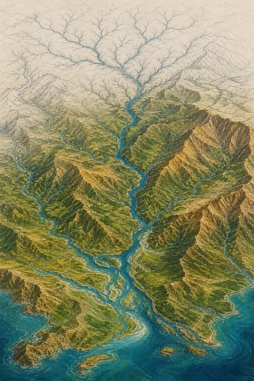
Terrain Generation Using Procedural Models Based on Hydrology

1. Terrain Generation Using Procedural Models Based on Hydrology

Jean-David Gnevaux¹

ric Galin^1*

ric Gurin¹

Adrien Peytavie¹

Bedřich Bene²

¹ Universit de Lyon, LIRIS, CNRS, UMR5205, France

² Purdue University, USA

Figure 1 consists of four panels. Panel A shows a 2D diagram of a terrain patch with a river network, labeled 'Terrain slope control'. Panel B shows a 2D diagram of a terrain patch with a river network, labeled 'River slope control'. Panel C shows a 3D visualization of a terrain patch. Panel D shows a 3D visualization of a river network.

Figure 1: A) Diagram showing terrain slope control with a patch and river network. B) Diagram showing river slope control with a patch and river network. C) 3D visualization of a terrain patch. D) 3D visualization of a river network.

Figure 1: A) The shape of a terrain is defined by a terrain patch and two functions that control the slope of rivers and valleys. B) The river network is automatically calculated and C,D) all inputs are then used to generate the continuous terrain conforming to rules from hydrology.

1.1. Abstract

We present a framework that allows quick and intuitive modeling of terrains using concepts inspired by hydrology. The terrain is generated from a simple initial sketch, and its generation is controlled by a few parameters. Our terrain representation is both analytic and continuous and can be rendered by using varying levels of detail. The terrain data are stored in a novel data structure: a construction tree whose internal nodes define a combination of operations, and whose leaves represent terrain features. The framework uses rivers as modeling elements, and it first creates a hierarchical drainage network that is represented as a geometric graph over a given input domain. The network is then analyzed to construct watersheds and to characterize the different types and trajectories of rivers. The terrain is finally generated by combining procedural terrain and river patches with blending and carving operators.

CR Categories: I.3.5 [Computer Graphics]: Computational Geometry and Object Modeling; I.3.6 [Computer Graphics]: Methodology and Techniques—Interaction Techniques I.6.8 [Simulation and Modeling]: Types of Simulation—Visual

Keywords: procedural modeling, terrain generation, hydrology

Links: DL PDF WEB VIDEO

*e-mail:eric.galin@liris.cnrs.fr

ACM Reference Format
Gnevaux, J., Galin, E., Gurin, E., Peytavie, A., Bene, B. 2013. Terrain Generation Using Procedural Models based on Hydrology. ACM Trans. Graph. 32, 4, Article 143 (July 2013), 10 pages.
DOI = 10.1145/2461912.2461996 http://doi.acm.org/10.1145/2461912.2461996.

Copyright Notice
Permission to make digital or hard copies of all or part of this work for personal or classroom use is granted without fee provided that copies are not made or distributed for profit or commercial advantage and that copies bear this notice and the full citation on the first page. Copyrights for components of this work owned by others than ACM must be honored. Abstracting with credit is permitted. To copy otherwise, or republish, to post on servers or to redistribute to lists, requires prior specific permission and/or a fee. Request permissions from permissions@acm.org.
Copyright ACM 0730-0301/13/07-ART143 $15.00.
DOI: http://doi.acm.org/10.1145/2461912.2461996

1.2. 1 Introduction

Virtual terrains have an important role in computer graphics, and their applications range from landscape design and flight simulators to movies and computer games. A terrain is the dominant visual element of the scene, or it plays a central part in the application.

Researchers have made considerable progress toward developing efficient methods for synthetic terrain generation. Existing techniques can be roughly classified into procedural, physics-based, and sketch- or example-based. Procedural methods, as well as physics-based algorithms, often lack controllability. Sketch-based methods involve manual editing that can be tedious. Example-based algorithms are limited by the provided input. Moreover, only the physics-based algorithms provide results that are correct from the standpoint of geology. Probably the most important problem in terrain generation for the field of computer graphics is the absence of algorithms that would allow the quick generation of controllable, and geologically reliable outputs. A related problem is the scalability of existing algorithms. The generated terrains usually represent only features of a single scale that are stored in a simple regular height field that becomes the standard data representation in many terrain-modeling systems. The height field is later converted into a mesh suitable for fast visualization with varying levels of details.

A key observation when looking at real terrains is that their morphologies are structured around river networks. Those networks subdivide the terrain into visual and clearly defined areas. Moreover, the geometric and visual properties of water-courses are nearly independent of the tectonic attributes and the climate [Rosen 1994], and they look identical at different scales independent of geological and climatic factors [Rodrguez-Iturbe and Rinaldo 1997; Dodd and Rothman 2000]. The rivers form a graph on the terrain surface and partition it into patches.

We propose a novel procedural approach, using river networks, for terrain modeling. The user optionally defines the river mouths and sketches the most important rivers on the terrain, and our approach generates the complete river network with the corresponding terrain, as shown in Fig. 1. The user can also control the river network and terrain generation with a set of intuitive parameters. Our method can represent large terrain models with complex river networks and geomorphologically consistent patterns that conform with observations from landscape and river science and yet provide a high level of controllability. The actual river geometry is generated by converting the drainage network data into a subset of river types that are taken from a well-known classification in hydrology [Rosen 1994]. The terrain is stored in a novel hierarchical continuous data representation that is inspired by constructive solid geometry (CSG). The terrain features are stored in the tree leaves, and the internal nodes define operations (blending, subtraction) on them. Contrary to most of the previous work, our terrain is represented by an analytic continuous function and not as a raster-based height field. Yet, our terrain is composed of many primitives and not a single abstract function. This allows us to generate large-scale terrains with an unlimited and locally varying level of detail.

The main contributions of our work are:

• an intuitive framework for procedural terrain generation using rivers as modeling features;
• a technique for terrain generation that is inspired by and that follows methods used in hydrology, but it also has the advantages of procedural approaches;
• a novel hierarchical hybrid terrain data representation that allows efficient terrain definition, editing, and visualization.

The paper continues with a review of previous work. Section 3 provides a high-level overview of the system. The following Section 4 describes details about the river generation, and Section 5 describes details about creation of the construction blocks and the CSG-like data structure. Section 6 and Section 7 show how the actual mesh representing terrain is generated, and the paper ends with results in Section 8 and conclusions and future work in Section 9.

1.3. 2 Related Work

Procedural techniques are a popular choice in computer graphics because of the simple implementation and wide range of terrains they provide when a few parameters are changed. One of the most important algorithms is the adaptive subdivision introduced by [Fournier et al. 1982], which provides an intrinsic level of detail. Noise-based procedural approaches, such as the Perlin noise [Perlin 1985], provide varying details by combining noise functions at various scales (see [Ebert et al. 1998] for an in-depth overview). Fractal-based methods produce large-scale terrains with unlimited detail, but they often lack control over the placement of terrain features, such as rivers and valleys. Furthermore, they provide terrains that look geologically fresh, whereas real terrains are usually affected by erosion and weathering.

Various techniques exist that attempt to incorporate rivers into the procedural terrain generation. Probably the first one is the paper by Kelley et al. [1988], who proposed a procedural method to generate watersheds. Their approach resembles ours because the river network is generated first and the terrain second. However, our algorithm creates large terrains represented by a continuous procedural model from a hydrographically and geomorphologically consistent river drainage network. It can also be used to generate terrains from partial input sketches. Prusinkiewicz et al. [1993] combined context-sensitive L-systems with the midpoint displacement method in an approach that imprints the rivers into fractal terrains. Later Belhadj and Audibert [2005] presented a modified stochastic subdivision algorithm that constrains ridges and river curves generated by fractional Brownian motion. Teoh [2009] presented an algorithm for terrain generation that also starts by producing the river network. However, our approach is based on models from hydrology, provides better control over the terrain generation process, and generates implicit terrain decomposition into continuous patches. Similarly, Derzapf et al. [2011] generated river networks on a planetary scale.

The above-mentioned algorithms provide river networks and watersheds that are not coherent, and the river paths are created with stochastic techniques that do not conform to the characteristics of rivers as observed in geomorphology. Moreover, these algorithms allow a user control limited to setting a few abstract parameters.

Physics-based techniques provide the foundations for the generation of terrains that are exposed to various morphological agents, such as water, temperature changes, or human activities. This has been addressed in the seminal paper [Musgrave et al. 1989]; in which a simple erosion-deposition model for hydraulic and thermal erosion was introduced. This approach has been extended in many different directions, such as [Nagashima 1998; Chiba et al. 1998; Bene and Forsbach 2002], who provided different thermal and hydraulic erosion algorithms.

Although most of the above-described techniques use regular height fields, layered data structures have been combined with erosion in [Bene and Forsbach 2001] and the same authors later introduced a full 3D volumetric hydraulic erosion in [Bene et al. 2006]. Smoothed particle hydrodynamics were combined with erosion in [Kritof et al. 2009], and corrosion simulation has been introduced in [Wojtan et al. 2007]. One of the main disadvantages of morphological algorithms is their low controllability. These methods also cannot model large terrains with a high level of detail, even though this problem has been partially alleviated by the recent GPU-oriented approaches [Mei et al. 2007; Vanek et al. 2011].

Interactive editing addresses the issue of controllability of the above-mentioned techniques. Rusnell et al. [Rusnell et al. 2009] used feature-based generation techniques, and the approach of [Zhou et al. 2007] used 2D height field examples, combining them into the final terrain. The approach leads to impressive results; however, as with every template-based algorithm, it fails to generate results that are not exemplified by the input.

Interactive terrain editing [Peytavie et al. 2009] and sketching approaches [Gain et al. 2009] provide good control over the resulting terrain, but they can lead to results that are not geologically correct. Hybrid approaches that attempt to combine interactive editing with physics-based algorithms [tava et al. 2008; Vanek et al. 2011] are limited to editing existing terrains and work only for small scenes.

Recently, Hnaidi et al. [2010] introduced an algorithm for a direct manipulation of river trajectories using vector-based models. Given a set of control curves representing landform features, such as ridge lines, cliffs, and riverbeds, the terrain is generated so that it matches the elevation and gradient constraints attached to the curves by using a multi-grid diffusion equation. Although this approach has the potential to provide large-scale realistic terrains, it does not address the geomorphological properties of a river-network creation.

1.4. 3 Algorithm Overview

An overview of the framework we propose is depicted in Fig. 2. In the first step, the user interactively provides the contour of the generated terrain, river mouths, some river parts, and input parameters.

From this input, the system first generates the drainage river network. The network is created inside the domain formed by the contour and is represented as a geometric graph. The graph is generated by a progressive growth from the seeds placed on the domain contour and the input rivers already sketched by the user. The expansion algorithm is inspired by Horton-Strahler's ordering [Horton 1945], which quantifies the complexity of a tree structure.

The output of the river network generator is a set of 3D polylines with increasing elevation from the outlet to the spring. The rivers and their parts are then classified into distinct procedural primitives. We use building blocks such as junctions, springs, deltas, and river trajectories, for the final river rendering. This categorization is inspired by the Rosgen classification [Rosgen 1994], which is used in hydrology and geomorphology.

Figure 2: Overview of the terrain generation method. The process starts with 'Contour and river parts' and 'Control parameters' as input. These feed into 'River Network Generation', which produces a 'River Network Graph G'. This graph is then processed by 'River Classification' to create a 'Detailed watershed, crest lines and river description'. Finally, 'Model generation' leads to a 'Hierarchical terrain representation' which includes 'Carve', 'Blend', and 'Final terrain' stages, with sub-components for 'River', 'Hills', and 'Mountains'.

Figure 2: Overview of our terrain generation method. From the input contour and partial river sketches the system generates a complete river network. The graph is then classified into distinct cells that are used to complete the terrain and that are stored in a hierarchical representation.

Once the river network is defined, the algorithm extracts the graph topology and geometry that is used for the terrain generation in the next step. We decompose the terrain into a set of patches by computing the Voronoi cells corresponding to the nodes of the river graph. The algorithm then generates the hierarchical watershed structure by traversing the geometric graph and gathering information of the Voronoi cells. This step enables us to compute the area of the watersheds and subwatersheds and to evaluate the flow of the water-courses at every node in the graph.

The output is controlled by two user-defined maps. The river slope map drives the dendritic shape of the river and directs the Rosgen type of each river. The terrain slope map controls the location of mountains and flatlands. The crest and ridge elevations are obtained by combining the river elevation and the terrain slope information. Both maps are either user-defined (Fig. 1, Fig. 17) or generated procedurally (Fig. 18, Fig. 20).

In the last step, the algorithm gathers information from the previous steps and generates the continuous-terrain model. We propose a novel procedural terrain representation that defines the terrain as a construction tree. The leaves are parameterized primitives that define different terrain features, such as hills, mountains, valleys, and different types of rivers. The inner tree nodes combine the primitives by blending, adding, subtracting, or carving. This approach creates a memory efficient representation of large terrains, comprising numerous levels of details.

1.5. 4 River Network Generation

The river network covering the input domain is a geometric graph that is generated in two steps. First, the seed nodes are distributed on the boundary of the input contour and at the initial user-defined rivers (Section 4.1). The rivers are then generated by a progressive growth inside the domain (Section 4.2).

Notations. Let $\Omega$ denote the input domain and $\Gamma$ its contour (defined as a 2-D polyline). The algorithm creates a coverage of $\Omega$ by a set of trees denoted as $\mathcal{G}$ . A tree is defined by its set of nodes $\mathcal{N}_j$ and a set of edges $\mathcal{E}_j$ . Every node $N_i = (\mathbf{p}_i, s_i, \rho_i, \phi_i)$ has the position $\mathbf{p}_i$ , the priority index $s_i$ , the river type $\rho_i$ according to Rosgen classification [Rosgen 1994], and the flow $\phi_i$ . Every edge has a constant length $e$ that is defined by the user. We will refer to the set of all nodes and edges $\mathcal{N} = \cup_j \mathcal{N}_j$ and $\mathcal{E} = \cup_j \mathcal{E}_j$ , respectively.

Figure 3: Three stages of river network generation. Step 1 shows an initial contour and a partial river graph. Step 2 shows the river network being incrementally generated by growing the geometric graph. Step 3 shows the final river network. A legend indicates: open circle for River node, filled circle for River mouth, red line for Sketched, and blue line for Generated.

Figure 3: Given an initial contour $\Gamma$ and a partial river graph $\mathcal{G}$ (step 1), the river network is incrementally generated by growing the geometric graph over the domain $\Omega$ (steps 2 and 3).

1.5.1. 4.1 Initial Candidate Nodes

The first step consists of creating the set of initial candidate nodes that will be expanded later. The candidate nodes are located at the river mouths on the contour $\Gamma$ . Alternatively, if the user specified input sketches representing some parts of the rivers, the initial nodes are placed on their extremities and on regularly jittered sample locations along their paths as shown in Fig. 3. Each node has been assigned a priority index that defines its importance. Both the position and the priority index define the overall appearance of the resulting river network hierarchy.

The initial candidate nodes placement can be either controlled by the user or generated automatically by a set of heuristics. The automatic placement is inspired by the observations from geomorphology, where the river mouths of two large rivers are typically apart, and large river mouths and deltas are frequently found in concave parts of the contour [Dunne and Leopold 1978].

1.5.2. 4.2 River Network Generation

The river network is generated by incrementally growing and elevating the geometric graphs $\mathcal{G}$ using a probabilistic approach. The graph network has a set of candidate nodes $\mathcal{X}$ that is expanded using a selection algorithm and several rules. We iteratively perform the following three steps:

1. Node selection: choose a node denoted $N_{\mathcal{X}}$ from the set of candidate nodes $\mathcal{X}$ that will be expanded.
2. Node expansion: expand the candidate node $N_{\mathcal{X}}$ and perform geometric tests to verify that the new nodes $\{N\}$ are compatible with the previously created ones.
3. Node creation: update the list of candidate nodes $\mathcal{X}$ :

$\mathcal{X} \leftarrow (\mathcal{X} \setminus \{N_{\mathcal{X}}\}) \cup \{N\}.$

The graph $\mathcal{G}$ is also updated to take into account the new nodes $\{N\}$ . If any new node is not compatible with the previously created nodes, it is removed from the graph.

1.5.2.1. 4.2.1 Node Selection

The node that will be expanded is selected from the list of candidate nodes by using a heuristic that takes into account the node elevation and its priority index. Combining those two criteria allows a simultaneous creation of several hierarchical drainage networks competing for space. Moreover, modifying the relative importance of the node elevation and its priority index provides the user with a control over the network shape. If the priority index is preferred, the algorithm favors networks created from river mouths independent of their relative elevation. In contrast, when the node with the lowest elevation is selected, the algorithm first generates the drainage network in the lowlands (Fig. 5).

Figure 4: Node selection process. Left: A map showing a drainage network with candidate nodes (blue circles) and a selected node (red circle). Right: A scatter plot of Elevation (y-axis, 0 to 20) vs. Priority (x-axis, 0 to 4). A shaded region represents the selection criteria: nodes with elevation between z and z + ̑, and priority greater than or equal to z. Nodes 24, 14, 8, 6, and 4 are shown in the plot.

Figure 4: The node selection process is controlled by a weighting function that combines the node elevation and its priority index. The algorithm first selects candidate nodes within the range $[z, z + \zeta]$ , ( $z$ being the lowest altitude of the candidate) then the one with the highest priority, and then the smallest elevation.

Let us recall that the $\mathcal{X} \subset \mathcal{N}$ denotes the set of candidate nodes created in the graph $\mathcal{G}$ during one expansion step. Our method proceeds as follows (Fig. 4):

1. find the elevation $z$ of the lowest located candidate;
2. consider the subset $\mathcal{X}_\zeta \subset \mathcal{X}$ of admissible nodes made of nodes whose elevations are within the range $[z, z + \zeta]$ ;
3. choose from the set of candidate nodes $\mathcal{X}_\zeta$ , the node $N_{\mathcal{X}}$ with the highest priority. If more than one candidate satisfies this criterion, the node with the lowest altitude will be chosen.

Figure 5: Two different drainage networks created from the same contour but with different parameters ̑. The left network is more compact and has a higher density of small branches, while the right network is more elongated and has fewer, larger branches.

Figure 5: Two different drainage networks created from the same contour but with different parameters $\zeta$ . When $\zeta = 0$ , we obtain networks of similar sizes, whereas one large drainage network and several small ones are generated with $\zeta = 20$ .

The parameter $\zeta \in [0; +\infty[$ controls the length of the drainage network by limiting the elevation range between two nodes $\mathcal{X}_\zeta$ (Fig. 5). For small values of $\zeta \approx 0$ , it prioritizes the nodes with the lowest elevation and causes rivers to have more ramifications. When $\zeta$ increases, the candidate node with the highest priority index is chosen, causing the formation of larger river-drainage networks.

1.5.2.2. 4.2.2 Node Expansion

River nodes are expanded using the rules described in Table 1. We use a grammar-like rewriting process that uses two nonterminal symbols denoted $\alpha$ and $\beta$ . The nonterminal symbols represent the candidate node and an instantiated node, respectively. The only terminal symbol $\tau$ represents a node that has been added to the graph and that cannot be further extended.

River Slope map. During the expansion step, the elevation of each new node should be higher than its ancestors to guarantee a consistent water flow. This elevation is computed according to a local river slope-magnitude value that is provided either by the user (Fig. 1 and 17) or generated procedurally (Fig. 18). Either way, the river slope-magnitude (a scalar value) defines only the height variation and provides no information on the direction of the expansion. Mapped on the whole terrain, this river slope map provides an intuitive way to describe how the drainage network will expand.

Index priority and Horton-Strahler's number. The nonterminal symbols in Table 1 are parameterized by an integer representing the priority index $s$ . This is the Horton-Strahler number [Horton 1945], which is a numerical measure of the branching complexity of the geometric graph representing the drainage network.

Figure 6: Horton-Strahler numbering. A diagram of a branching network where nodes are labeled with their Horton-Strahler number. The root node is labeled 1, and its children are labeled 2 and 3. The node labeled 3 has children labeled 1 and 2. The node labeled 2 has children labeled 1 and 1. The node labeled 1 has children labeled 1 and 1.

Figure 6: Horton-Strahler numbering.

The Horton-Strahler number of a leaf is $s = 1$ . The Horton-Strahler number $s$ of a node is equal to the inherited maximum number of its children $k$ except when two or more children are labeled with $k$ , then $s = k + 1$ .

The rules use the Horton-Strahler number evaluation and code it into a symmetric (rule 2.2) and an asymmetric (rule 2.3) branching. Because the priority index may decrease at every branching node, in some instances all the remaining candidate nodes may have the same priority index equal to one. Should that happen, the grammar relies on the first production rule, so the geometric graph will continue to grow on the domain $\Omega$ . The growth stops when it is no longer possible to add new nodes. If a node with a high priority cannot be expanded because of geometric constraints, all Horton-Strahler numbers are adjusted accordingly. Although we use Horton-Strahler rules for expansion, the approach is generic and could be replaced without changing the framework.

Rule application. The probabilities of the rule application $\mathcal{P}_c$ , $\mathcal{P}_a$ , $\mathcal{P}_s$ , with $\mathcal{P}_c + \mathcal{P}_a + \mathcal{P}_s = 1$ are defined by the user, and they influence the relative number of branching nodes in the final graph. The numbers $\mathcal{P}_a$ and $\mathcal{P}_s$ refer to the probability of occurrence of an asymmetric and a symmetric branching, respectively, whereas $\mathcal{P}_c$ denotes the probability of a simple continuation without branching.

Compatibility. If a new node should be added (rules 2.1–2.3), its compatibility with the already produced geometric graph is verified (rules 3.1 – 3.2). Invalid nodes are removed from the production by applying the $\varepsilon$ -rule (rule 3.2).

Let $N_{\mathcal{X}} \in \mathcal{N}$ denote the candidate node for expansion. Let $N = (\mathbf{p}, s, \rho, \phi)$ be the node that we try to add to the graph and $E$ be the edge $(N, N_{\mathcal{X}})$ . The length of the geometric edge is $e$ , and $N_i = (\mathbf{p}_i, s_i, \rho_i, \phi_i)$ are the nodes of $\mathcal{N}$ . The point $\mathbf{p}$ should be inside the domain and farther from the contour $\Gamma$ (Fig. 7) than the user-defined

0.			$\alpha_1(s_1) \dots \alpha_n(s_n)$	$\{ \textit{Axiom} \}$
1.	$\alpha(1)$	$\longrightarrow$	$\tau(1) \beta^p(1)$ with $p \in [1; 5]$	$\{ \textit{Filling} \}$
2.1	$\alpha(n)$	$\longrightarrow$	$\tau(n) \beta(n)$	$\{ \textit{River growth} \}$
2.2		$\longrightarrow$	$\tau(n) \beta(n-1) \beta(n-1)$	$\{ \textit{Symmetric Horton-Strahler junction} \}$
2.3		$\longrightarrow$	$\tau(n) \beta(n) \beta(m)$ where $m < n$	$\{ \textit{Asymmetric Horton-Strahler junction} \}$
3.1	$\beta(n)$	if valid	$\alpha(n)$	$\{ \textit{Instantiation: } \mathcal{X} \leftarrow (\mathcal{X} \setminus \{N_{\mathcal{X}}\}) \cup \{N\} \}$
3.2		otherwise	$\varepsilon$	$\{ \textit{Rejection: } \mathcal{X} \leftarrow \mathcal{X} \setminus \{N_{\mathcal{X}}\} \}$

Table 1: Expansion rules for the hierarchical drainage network growth.

value $\eta$ (we use $\eta = 3/4 e = 1500[\text{m}]$ in our implementation):

$\mathbf{p} \in \Omega \quad \wedge \quad d(\mathbf{p}, \Gamma) > \eta.$

We compute the distance between the edge $E$ and the other edges in the geometric graph to avoid collision between the new edge and the existing graph (Fig. 7): this distance should be greater than a user-defined limit denoted as $\sigma$ (we use $\sigma = 3/4 e = 1500[\text{m}]$ in our implementation). The function $\sigma \cdot f(s)$ depends on the Horton-Strahler number to maintain large rivers apart:

$\forall E_i \in \mathcal{E} \quad : \quad d(E, E_i) > \sigma \cdot f(s).$

The elevation of $\mathbf{p}$ should also be compatible with the elevation of

Figure 7: Contour and graph distance conditions. Two diagrams show a domain Omega with a river network. Diagram 1 shows a point p (green dot) where d(p, Gamma) > eta. Diagram 2 shows a point p (green dot) where d(E, E_i) > sigma. A legend indicates: yellow square for 'Invalid location', green circle for 'New node', blue circle for 'Existing node', and red circle for 'Parent node'.

Figure 7: Contour and graph distance conditions.

the other nodes and higher than its ancestor node $N_{\mathcal{X}}$ . We constrain the terrain generation so that the maximum local slope in the graph should be less than a given threshold $\kappa$ depending on the location of the point. The constant $\kappa$ represents an upper bound of the slope-mapping function. Therefore, we make sure that the new point $\mathbf{p}$ will satisfy the Lipschitz condition: $|\mathbf{p}_z - \mathbf{p}_z'| < \kappa(\mathbf{p}) \cdot d(\mathbf{p}, \mathbf{p}')$ . This condition prevents the creation of huge cliffs.

The effect of varying parameters on the generated river network is depicted in Fig. 8. The parameter set ( $P_c = 0.2, P_s = 0.7, P_a = 0.1$ ) produced highly curved watersheds (left). There are only a few main streams, but many ( $> 75\%$ ) small streams with a Horton-Strahler numbers equal to 1 (Fig. 8 left). In contrast, the parameter set ( $P_c = 0.2, P_s = 0.1, P_a = 0.7$ ) produced drainage networks with watersheds of comparable sizes (Fig. 8 right). In the second case, the main rivers are longer because their priority indices were statistically kept longer in the queue during the graph generation, and the watersheds are structured around this main river.

We quantified the difference (Fig. 8) between these two graphs by evaluating the number of edges in the graph with the same Horton-Strahler number and by comparing their relative frequencies. Whenever $P_s$ is high, the index of priority is very likely to decrease, whereas for high values of $P_a$ , the main streams will continue to grow longer and will have a stronger influence on the overall pattern of the watershed.

Figure 8: Two different drainage networks and their corresponding watersheds produced with two sets of parameters. The figure shows two bar charts and two maps. The left chart shows occurrences (%) for s=1, 2, 3, >4 with values 82, 10, 4, 4 respectively. The right chart shows occurrences (%) for s=1, 2, 3, >4 with values 59, 20, 10, 5 respectively. Below each chart is a map of a watershed with a river network. The left map corresponds to P_c=0.2, P_s=0.7, P_a=0.1 and the right map to P_c=0.2, P_s=0.1, P_a=0.7.

Figure 8: Two different drainage networks and their corresponding watersheds produced with two sets of parameters.

1.6. 5 River Classification

The river graph divides the domain $\Omega$ into nonoverlapping cells that allow us to build a set of watersheds and to construct a dual graph that stores crests (Section 5.1). The water flow is extracted from the river graphs, and each water-course is labeled with respect to the Rosgen classification (Section 5.2).

1.6.1. 5.1 Segmentation and Elevation of Crests

The domain $\Omega$ is decomposed into a set of cells $\mathcal{V} = \{V_i\}$ computed from the Voronoi diagram of node locations $\mathbf{p}_i$ . Some Voronoi cell boundaries correspond to the ridges that define the edges of the watersheds. Each cell vertex has an elevation assigned, and each cell $V$ is represented as a polygon composed of crest points $\mathbf{q}_i$ . Water entries are denoted $\mathbf{e}_0, \dots, \mathbf{e}_{n-1}$ , and the water outlet is denoted $s$ (see Fig. 10).

Figure 10: An example of watershed (in blue) and a Voronoi cell. The figure shows a map of a watershed with a river network. A specific watershed is highlighted in blue. To the right, a Voronoi cell is shown with vertices labeled q_0, q_1, q_2, q_3, q_4. Water entry points are labeled e_0, e_1, and the water outlet is labeled s.

Figure 10: An example of watershed (in blue) and a Voronoi cell.

Figure 9: Rosgen classification of water-courses. The figure shows nine panels labeled A+, A, B, C, D, DA, E, F, and G. Each panel displays a cross-section of a river channel with its characteristic shape and a corresponding longitudinal profile below it. The profiles show the river bed elevation relative to a datum. The river types range from simple, straight channels (A+, A) to complex, braided systems (D, DA) and highly meandering channels (E, F, G).

Figure 9: Rosgen classification of water-courses. Different river types depend on their water flow, elevation, distance from the spring, and other parameters. The final river is composed by procedurally connecting modified parts of the river blocks.

Watersheds are associated with each water outlet $s$ of a cell $V_j$ and are defined as the set of upstream connected cells $V_k \in V$ .

River flow evaluation contributes to the definition of the water-course. The exact computing is a complex problem that depends on multiple parameters, such as the climate and the soil composition.

We use a simplified model based on an empirical power law observed in geomorphology [Dunne and Leopold 1978]. Let $A$ [m²] be the watershed area. The mean flow $\phi$ of the river [m³s^-1] is given by $\phi = 0.42 \cdot A^{0.69}$ . The watershed area $A$ is approximated by the sum of the areas of cells connected to $s$ in the graph, and it allows calculation of the outgoing flow $\phi$ of any cell $V$ (Fig. 10). This equation takes into account evaporation and infiltration, and that is why the volume flow is not preserved.

Ridges. The computation of ridge elevation is important to guarantee a coherent flow. Each Voronoi cell has two types of edges: those that do not intersect the river graph and that define ridge lines, and those that carry a river entry $e_k$ or outlet $s$ .

Figure 11: Computation of the crest elevation. The diagram shows a Voronoi cell with three river nodes labeled a, b, and c. A crest point q is located at the intersection of the edges connecting these nodes. Distances d are indicated from the nodes to the crest point. The diagram illustrates how the crest point is determined based on the relative elevations of the nodes and their distances.

Figure 11: Computation of the crest elevation is based on the river nodes elevations.

Every crest point $q$ is located at an equal distance $d$ from the centers $a$ , $b$ , $c$ of three river nodes. This crest $q$ should have a higher elevation than $a$ , $b$ , and $c$ so that the water flows down consistently. We compute the elevation $q_z$ as

$q_z = \max(a_z, b_z, c_z) + \lambda(q) \cdot d,$

where $\lambda \in [0; 0.25]$ is another slope-magnitude function that describes if the terrain is mountainous. This terrain slope map can also be either generated

or given by the user. It describes which parts of the terrain will become plains, plateaus, valleys, or mountains. Further, this function can be weighted according to the distance to the coast and to the elevation of the nodes to generate either smoother valleys or sharp features as in cliffs.

1.6.2. 5.2 Water-courses Labeling

After the domain is segmented, we classify the water-course presented in every Voronoi cell $V_i$ . Our method relies on the Rosgen classification [Rosgen 1994] that defines nine river categories depending on their slopes and trajectories. Each river class has a trajectory type (A+, A, B, C, D, DA, E, F, or G) and a digging profile of the riverbed (Fig. 9). The classification includes the geological composition of the riverbed (bedrock, rocks, stones, gravel, sand, silt, or clay) in this description.

We assign to each river node its classification based on the slope of the river and its proximity to the coast. River nodes that are close to coasts (based on a geodesic distance threshold) are labeled as braided rivers (those consisting of multiple channels separated by bars and defined as D or DA). Similarly, river mouths with a flow greater than a fixed value are marked as deltas.

The type of every river edge is calculated from its two nodes, and junction types are determined by a look-up table. Rivers and meanders are generated by functionally defined river primitives. The parameters that define the river geometry depend on the input and output flows so that river primitives connect seamlessly.

1.7. 6 Terrain Model Generation

The mesh generation step uses the above-described procedural representation to build the final terrain model from its components: network graph, flow data $\phi$ , and node type $\rho$ .

The river primitives generation proceeds in two steps. First, for every Voronoi cell $V$ , we build river junctions and refine river paths according to type (Section 6.1). Second, we compute a set of terrain primitives that covers the cell domain $V$ (Section 6.2).

1.7.1. 6.1 River Primitives Generation

The river primitives generation proceeds in two steps: river junctions in a single cell $V$ are built, and then the precise paths of rivers are refined by subdivisions with respect to their Rosgen type.

Junction creation defines the river junctions inside a cell. A single cell $V$ has exactly one outlet (downstream), and 0- $n$ water entries (upstream). The hydrographics network is created by incremen-

Figure 12: Incremental junction generation algorithm. The diagram shows two stages of junction generation within a Voronoi cell V. The first stage, 'First junction made with the inputs', shows a cell with multiple input edges e1, e2, ..., en and one output edge s. A junction k0 is formed by connecting the inputs. The second stage, 'Second junction and link toward the output', shows the next junction k1 formed by adding a new input edge e0 to the previous junction. The output edge s is now the link from the final junction k1.

Figure 12: Incremental junction generation algorithm.

tally forming $n - 1$ confluences inside the cell $V$ (denoted $k$ in Fig. 12). The process starts with two neighboring water entries on the contour of $V$ . We denote the first confluence $k_0$ . Each water entry is then connected incrementally to the last created confluence. The connection angle is computed for each junction, depending on the position and water flow of the input rivers. When the junction involves two rivers having significantly different water flows (and thus two different Horton-Strahler numbers), the connection angle is set to be nearly perpendicular. Similarly, junction of two rivers of the same size will cause a small angle. Once the junctions are built,

Figure 13: A map showing different trajectories of rivers corresponding to their Rosgen type. The map features a network of river segments in light blue, medium blue, and dark blue, connected at various angles. The segments are labeled with letters B, G, and D, representing different river types.

Figure 13: Different trajectories of rivers corresponding to their Rosgen type. Light blue is type B, blue type G, and dark blue D.

we refine river paths with respect to their type. They are subdivided into subpaths of lengths lower than a user-defined parameter. Positions and tangents of the new curves are randomly perturbed to create a variety of windings according to their type (Fig. 13).

1.7.2. 6.2 Terrain Primitives Generation

The terrain is generated by blending a set of compactly supported fragments on which rivers are carved. To do this, we need a set of primitives $\{T\}$ covering $V$ with assigned parameters. Points

Figure 14: A diagram illustrating terrain primitive distribution and elevation. It shows a Voronoi cell with a river segment (a) and its projection on the ridge lines (b). The altitude of each primitive is based on the crest heights that are derived from the terrain slope map and the river node altitude.

Figure 14: Terrain primitive distribution and elevation.

are generated by semistochastic sampling using Poisson distribution [Lagae and Dutré 2005] that assures aperiodic tiling (Fig. 14 left). Disks' radii are increased until the set of primitives $\{T\}$ covers $\Omega$ . We used 50 samples per cell. Fewer samples give fast and memory inexpensive models but produce less accurate terrain.

In the next step, the elevation of the primitive centered around $c$ is calculated as a distance-weighted combination of elevations. We use two points for this combination: the projection of the point on the set of rivers ( $a$ ) and its projection on the ridge lines of the Voronoi cell ( $b$ ) (Fig. 14 right). The altitude of each primitive is based on the crest heights that are derived from the terrain slope map and the river node altitude.

The shape of the terrain is modulated by a random noise. The noise attributes (amplitude, frequency) associated with the primitives are calculated with respect to the distance to the river $d_a$ and the elevation differences between the river $a_z$ and crests $b_z$ . This modulation produces more roughness for the mountains than for the valleys. Using noise can produce small local minima, but they remain negligible in the context of large-scale hydrology.

1.8. 7 Terrain Tree Definition

The terrain is stored in a novel hierarchical representation where its surface is defined procedurally as a continuous function $h(\mathbf{p}) : \Omega \rightarrow \mathbf{R}$ . We define $h$ using a construction tree whose leaves are

primitives describing terrain fragments, and the inner nodes combine subtrees together. In this way, the elevation of a point can be defined as a combination of a hierarchy of primitives. Our approach

Figure 15: A diagram showing the construction of a terrain patch. It starts with a 'River' primitive (a green line on a brown background) and a 'Mountain' primitive (a brown sphere). These are combined in a 'Blend' step to create a 'Hill' primitive (a brown sphere with a green line). Finally, the 'Hill' primitive is combined with another 'Mountain' primitive in a 'Carve' step to create the 'Final terrain' (a brown surface with a green line).

Figure 15: Tree representing a river carved into a terrain patch.

was inspired by the Constructive Solid Geometry and by the Blob-Tree model [Wyvill et al. 1999]. However, in our model, every tree node defines two functions: $h(\mathbf{p})$ controls the elevation of the point, and $w(\mathbf{p})$ defines the influence field for the considered node and allows for complex combinations.

We define four node types: terrain $T$ and river $R$ primitives, and blending $B$ and replace $C$ operators. The construction tree (Fig. 15) describes the blending of terrain fragments $\{T_i\}$ on which the rivers' primitives $\{R_i\}$ are carved. Formally, the whole tree is defined as $\mathcal{A} = C(B(\{T_i\}), B(\{R_i\}))$ .

Figure 16: A diagram illustrating terrain and river primitives. The left part shows a river primitive with a center point c, a radius r, and a point p. The right part shows a terrain primitive with a center point c, a radius r, and a point p. The distance from p to the river skeleton is denoted as d(p), and the distance from p to the terrain skeleton is denoted as delta(d(p)).

Figure 16: Example of terrain and river primitives.

Primitives are defined by a geometric skeleton (point, segment, curve) and a set of parameters that describe elevation and weighting functions. Weighting functions $w(\mathbf{p})$ of primitives are defined on a compact support to limit their influence. Let $d(\mathbf{p})$ denote the distance to the skeleton of a primitive. We define:

$w(\mathbf{p}) = \frac{(1 - d(\mathbf{p})^2)^2}{r^4} \text{ if } d(\mathbf{p})^2 < r^2 \text{ else } w(\mathbf{p}) = 0.$

Terrain primitives $T$ have a center $c$ and a radius $r$ that describe their areas of influence (Fig. 16 left). We also use Perlin noise [Perlin 1985] as $n(\mathbf{p})$ to control the local soil roughness. We define:

$h(\mathbf{p}) = c_z + n(\mathbf{p})$

Each river primitive $R_i$ is built from a curve skeleton that defines the river path $\gamma$ and from a river profile function $\delta$ that describes the river profile perpendicular to the curve (Fig. 16 right). We use a set of profiles $\{\delta\}$ . Each profile is stored as a one-dimensional piecewise function that corresponds to the river type. The profile can be made of multiple layers that correspond to bedrock, water, and sand. The signed distance between $\mathbf{p}$ and the curve $\gamma$ is denoted $d(\mathbf{p})$ , and the projection of $\mathbf{p}$ on $\gamma$ is denoted $u(\mathbf{p})$ . We define

$h(\mathbf{p}) = u_z(\mathbf{p}) + \delta(d(\mathbf{p}))$

Primitives describing confluences or multiple river streams are built in the same way, but with more complex skeletons.

Figure 17: Two different terrains and their corresponding constraint maps. The figure shows two sets of terrain generation. Each set includes a 'Terrain slope control' map (A 1 and A 2), a 'River slope control' map (A 3 and A 4), and the resulting terrain (B 1 and B 2). The terrain B 3 is also shown. The constraint maps use color to represent different slope values, and the resulting terrain shows the generated topography.

Figure 17: Two different terrains and their corresponding constraint maps.

Operator nodes combine elevations and weighting of two subnodes denoted A and B. The blending of A and B, denoted $B(A, B)$ , combines elevation functions $h_A$ and $h_B$ with respect to the weighting functions $w_A$ and $w_B$ and allows the blending and joining of two terrain primitives.

$h_{B(A,B)} = \frac{w_A h_A + w_B h_B}{w_A + w_B} \quad w_{B(A,B)} = (w_A + w_B)/2$

The replacement operator $C(A, B)$ continuously replaces terrain A with terrain B. This asymmetric operator is used to place water-course geometry onto the terrain:

$h_{C(A,B)} = (1-w_B) h_A + w_B h_B \quad w_{C(A,B)} = (1-w_B) w_A + w_B^2$

1.9. 8 Results

We have implemented our system in C++. Experiments have been performed on a desktop computer equipped with Intel^® Core i7, clocked at 3 GHz with 16GB of RAM. The output of our system was directly streamed into MentalRay^® to produce photorealistic images (Fig. 20, 22).

Evaluation. Our procedural approach can generate large terrains that have a piecewise fractal structure with distinct river networks (Fig. 18) results that are difficult to achieve using traditional fractal or erosion-based techniques. The phenomenological approach is based on hydrological observations and allows us to obtain the structure of valleys at large scales by the means of Horton-Strahler-based rules as well as detailed geometry assets by using the Rosgen classification.

Figure 18: Example of a structured terrain with valleys and rivers. The image shows a top-down view of a terrain with a network of blue lines representing rivers and valleys, overlaid on a textured, brownish terrain.

Figure 18: Example of a structured terrain with valleys and rivers.

We have attempted to recreate a model of an existing island using our approach as shown in Fig. 19. Having a given example, we have defined interactively the main domain and sketched the principal river streams. The system then automatically completed the terrain. The results are visually similar though they are not exact because of the stochastic nature of our algorithm. The overall time necessary to create the input slope maps was less than five minutes. Default parameters were used to generate these images.

Control. One of the main contributions of our approach is its simplicity and the modular pipeline which allows us to control every step of the process. This control can be used to guide some features (river mouth definition, sketching rivers, river priority changing) or to choose which river will be salient. An intuitive user control can

Figure 19: The user sketched two constraint functions in two minutes (A) and our system completed the terrain. The figure shows four panels: A (sketch of river and mountain constraints), B (resulting terrain with river network), C (terrain with mountain location), and D (realistically looking terrain D).

Figure 19: The user sketched two constraint functions in two minutes (A) and our system completed the terrain. The output share similar water-courses trajectories (B) and mountain location (C) with a realistically looking terrain (D).

be achieved by sketching both river and terrain slope maps : this way, the user can sketch mountain and valley areas. Independently on the quality of the user input, our approach will lead to a hydrographically correct river network as shown in Fig. 1 and 17.

Performance. Our method generates a vector-based representation of large terrains (several hundreds of square kilometers) in a few seconds (Table 2) and, though it is based on principles from hydrology, it does not rely on complex numerical physics-based simulations. The novel description of the generated terrain

Table 2: Computation time [s] for the graph generation (1), flows and watershed computation (2), the tree construction, (3) and the evaluation ( $1024 \times 1024$ samples) of the tree into a 3D mesh (4).

	Graph (1)	Cells (2)	Tree (3)	Mesh (4)
Fig.17 A	4.0	0.9	4.7	1.0
Fig.17 B	5.3	1.1	4.9	1.2
Fig.18	0.1	0.1	1.8	1.0
Fig.19	0.2	0.2	4.2	0.7
Fig.20	0.6	0.4	4.6	1.0
Fig.22	0.5	0.4	4.8	0.8

has native multiresolution support. We can visualize the terrain at multiple scales, and we can use view-dependent clipping algorithms or resource-dependent strategies. The vector-based primitive description of the generated terrain is compact (average of $1 \text{ km}^2 \approx 1.5 \text{ kB}$ ) and allows the storage of large terrains as shown in Table 3. Even if the construction tree describe the whole domain, the user can evaluate only a portion of the landscape. Hoya Island (Fig 17-B) has an area of $3368 \text{ km}^2$ and is composed of 81853 primitives using 8,180 kB. A $30 \text{ km}^2$ portion of the terrain represents only 2068 primitives and a 225 kB storage.

Figure 20: Three side-by-side landscape renderings showing a lowland river with junctions in a valley. The terrain is green with scattered trees and a winding river path.

Figure 20: Example of a lowland river with junctions in a valley.

Table 3: Terrain statistics: domain size (km²), hydrographic network length (km) and number of construction primitives used.

	Terrain size [km²]	Network length [km]	Primitives
	Terrain size [km²]	Network length [km]	Terrain	Rivers
Fig.17 A	3055	1978	69065	4905
Fig.17 B	3368	2106	76332	5321
Fig.18	970	399	18941	885
Fig.19	2482	973	46435	2183
Fig.20	3386	1686	68956	3775
Fig.22	3050	1515	62205	3465

Limitations. The main limitation of our approach is that it can generate only terrains that were once subject to hydraulic erosion. A dry terrain can be simulated by not-adding the river beds and a geological fresh terrain is simply a single fractal patch. Another limitation is that the river network can subdivide only upstream; thus our algorithm cannot represent deltas or oxbow lakes. Specific geometric primitives could generate these features but only on a small scale.

Another limitation comes from the greedy construction that can lead to meandering crests and outcroppings of unnatural-looking hills. The Lipschitz condition reduces this problem, even if generated terrains sometimes lack soft transitions between plains and mountainous terrains, but does not solve this problem entirely. Also, the generated river network cannot easily adapt to large mountains with clearly articulated valleys. If the slope maps have strong variations flat rivers can cut through high mountains. Our method has a large amount of parameters that allows us to create unnatural terrains. The balance between the user control and the system control could be addressed as future work.

1.10. 9 Conclusion

We introduced a novel hydrology-based method for procedural terrain generation that allows a high level of control of the generation process. The terrain generation is derived from the underlying hydrographic network, and it guarantees that the construction satisfies hydrographic properties. The final geometric model is made of vector-based primitives and is able to describe hills, mountains, valleys, and water-courses with highly detailed geometry on varying scales. The key motivation for our work comes from the Rosgen classification in hydrology that allows us to produce important visual features of rivers, such as paths and profiles. There are many possible extensions of this work. As with every procedural system, the rules and the labeling algorithm require a certain level of experimentation to find a set of well-behaving values. However, the values presented in this paper led to visually plausible terrains

$Figure 21: A 2x2 grid of terrain renderings. Top-left: 'Erosion simulation' showing a smooth, eroded landscape. Top-right: 'Our method' showing a more complex, layered terrain. Bottom-left: 'Fractal generation' showing a highly detailed, fractal-like terrain. Bottom-right: 'Real dataset' showing a real-world terrain with complex features.$

Figure 21: A 2x2 grid of terrain renderings. Top-left: 'Erosion simulation' showing a smooth, eroded landscape. Top-right: 'Our method' showing a more complex, layered terrain. Bottom-left: 'Fractal generation' showing a highly detailed, fractal-like terrain. Bottom-right: 'Real dataset' showing a real-world terrain with complex features.

Figure 21: Visual comparison of terrains produced using different algorithms; erosion was simulated using [Štáva et al. 2008]. Our approach has features from lowlands to mountains that are difficult to achieve with traditional approaches.

(Fig. 21). The speed of the method provides simplified modeling and interactive editing. Another possible extension would be to include the generation of vegetation straight in the same process. We could, for example, automatically generate the distribution of trees and vegetal species on the terrain, especially along the rivers. Our system is based on the behavior observed in hydrology. It would be interesting to adapt our approach to the simulation of urban areas combined with rivers.

1.11. References

BELHADJ, F., AND AUDIBERT, P. 2005. Modeling landscapes with ridges and rivers: bottom up approach. In GRAPHITE, 447–450.
BENEŠ, B., AND FORSBACH, R. 2001. Layered data representation for visual simulation of terrain erosion. In Proc. of the Spring Conf. on Comp. Graphics, 80–85.
BENEŠ, B., AND FORSBACH, R. 2002. Visual simulation of hydraulic erosion. In Journal of WSCG, vol. 10, 79–86.
BENEŠ, B., TEŠŇSKÝ, V., HORNÝŠ, J., AND BHATIA, S. 2006. Hydraulic erosion. Comp. Anim. Virt. Worlds 17, 2, 99–108.
CHIBA, N., MURAOKA, K., AND FUJITA, K. 1998. An erosion model based on velocity fields for the visual simulation of mountain scenery. Journal of Vis. and Comp. Anim. 9, 4, 185–194.
DERZAPF, E., GANSTER, B., GUTHE, M., AND KLEIN, R. 2011. River networks for instant procedural planets. Comput. Graph. Forum 30, 7, 2031–2040.

Figure 22: Five computer-generated images of a braided river in arid highlands at different levels of detail. The top-left image shows a wide view with a large mountain in the background. The top-right image is a closer view of the river's braided channels. The bottom-left image shows a more detailed view of the river's banks and vegetation. The bottom-middle image is a close-up of the river's surface and banks. The bottom-right image shows a different view of the river's braided channels.

Figure 22: Different views of a braided river in arid highlands at different levels of detail.

DODD, P., AND ROTHMAN, D. 2000. Scaling, universality, and geomorphology. Annual Review of Earth and Planetary Sciences 28, 571610.
DUNNE, T., AND LEOPOLD, L. B. 1978. Water in Environmental Planning. W.H. Freeman.
EBERT, D., MUSGRAVE, K., PEACHEY, D., PERLIN, K., AND WORLEY, S. 1998. Texturing and Modeling: A Procedural Approach. Academic Press Professional.
FOURNIER, A., FUSSELL, D., AND CARPENTER, L. 1982. Comp. rendering of stochastic models. Comm. ACM 25, 6, 371–384.
GAIN, J., MARAIS, P., AND STRASSER, W. 2009. Terrain sketching. In Proc. of Interactive 3D graphics and games, 31–38.
HNAIDI, H., GURIN, E., AKKOUCHE, S., PEYTAVIE, A., AND GALIN, E. 2010. Feature based terrain generation using diffusion equation. Comp. Grap. Forum 29, 7, 2179–2186.
HORTON, R. E. 1945. Erosional development of streams and their drainage basins: hydro-physical approach to quantitative morphology. Geological Society of America Bulletin 56, 3, 275370.
KELLEY, A., MALIN, M., AND NIELSON, G. 1988. Terrain simulation using a model of stream erosion. In Computer Graphics 22, 4, 263–268.
KRISTOF, P., BENE, B., KRIVNEK, J., AND TAVA, O. 2009. Hydraulic erosion using smoothed particle hydrodynamics. Comp. Grap. Forum 28, 2, 219–228.
LAGAE, A., AND DUTR, P. 2005. A procedural object distribution function. ACM Trans. Graph. 24, 4 (Oct.), 1442–1461.
MEI, X., DECAUDIN, P., AND HU, B. 2007. Fast hydraulic erosion simulation and visualization on GPU. In Pacific Graphics, 47–56.
MUSGRAVE, F. K., KOLB, C. E., AND MACE, R. S. 1989. The synthesis and rendering of eroded fractal terrains. In Computer Graphics 23, 3, 41–50.
NAGASHIMA, K. 1998. Computer generation of eroded valley and mountain terrains. The Visual Computer 13, 9–10, 456–464.
PERLIN, K. 1985. An image synthesizer. In Computer Graphics 19, 3, 287–296.
PEYTAVIE, A., GALIN, E., MERILLOU, S., AND GROSJEAN, J. 2009. Arches: a Framework for Modeling Complex Terrains. Comp. Grap. Forum 28, 2, 457–467.
PRUSKIEWICZ, P., AND HAMMEL, M. 1993. A fractal model of mountains with rivers. In Graphics Interface, 174–180.
RODRIGUEZ-ITURBE, I., AND RINALDO, A. 1997. Fractal River Basins: Chance and Self-Organization. Cambridge Univ. Press.
ROSGEN, D. L. 1994. A classification of natural rivers. Catena 22, 169–199.
RUSNELL, B., MOULD, D., AND ERAMIAN, M. G. 2009. Feature-rich distance-based terrain synthesis. The Visual Computer 25, 5-7, 573–579.
TEOH, S. T. 2009. Riverland: An efficient procedural modeling system for creating realistic-looking terrains. In Proc. of the Int. Symp. on Advances in Visual Computing: Part I, 468–479.
VANEK, J., BENE, B., HEROUT, A., AND TAVA, O. 2011. Large-scale physics-based terrain editing using adaptive tiles on the GPU. Comp. Graphics and App., IEEE 31, 6, 35–44.
TAVA, O., BENE, B., BRISBIN, M., AND KRIVNEK, J. 2008. Interactive terrain modeling using hydraulic erosion. In Symposium on Computer Animation, 201–210.
WOITAN, C., CARLSON, M., MUCHA, P., AND TURK, G. 2007. Animating corrosion and erosion. In Proc. of the Eurographics Workshop on Natural Phenomena, 15–22.
WYVILL, B., GUY, A., AND GALIN, E. 1999. Extending the csg tree - warping, blending and boolean operations in an implicit surface modeling system. Comp. Grap. Forum 18, 2, 149–158.
ZHOU, H., SUN, J., TURK, G., AND REHG, J. M. 2007. Terrain synthesis from digital elevation models. IEEE Transactions on Visualization and Computer Graphics 13, 4, 834–848.