Responsive Real-Time Grass Rendering for General 3D Scenes

1. Responsive Real-Time Grass Rendering for General 3D Scenes

Klemens Jahrmann*
TU Wien

Michael Wimmer†
TU Wien

A 3D rendering of a grassy field with a large, colorful, translucent bunny-like object on the left. A bowling ball is rolling on the grass, and its trail is visible in wireframe mode. In the background, there are trees and a cloudy sky.

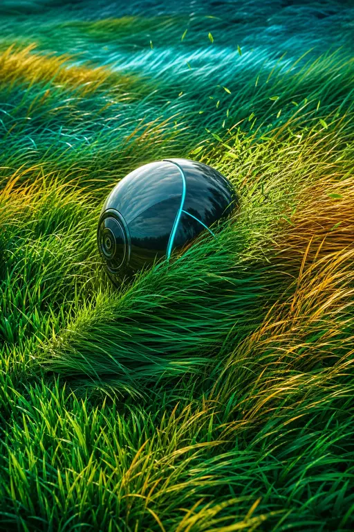
Figure 1: This figure shows an example of our rendering technique. The collision reaction is visible at the trail of the bowling ball. The right side is rendered in wireframe mode to show the accuracy of our occlusion culling method.

1.1. Abstract

Grass plays an important role in most natural environments. Most interactive applications use image-based techniques to approximate fields of grass due to the high geometrical complexity, leading to visual artifacts. In this paper, we propose a grass-rendering technique that is capable of drawing each blade of grass as geometrical object in real time. Accurate culling methods together with an adaptable rendering pipeline ensure that only the blades of grass that are important for the visual appearance of the field of grass are rendered. In addition, we introduce a physical model that is evaluated for each blade of grass. This enables that a blade of grass can react to its environment by calculating the influence of gravity, wind and collisions. A major advantage of our approach is that it can render fields of grass of arbitrary shape and spatial alignment. Thus, in contrast to previous work, the blades of grass can be placed on any 3D model, which is not required to be a flat surface or a height map.

Keywords: real-time rendering, vegetation, hardware tessellation

Concepts: •Computing methodologies → Rendering; Physical simulation; Visibility;

1.2. 1 Introduction

Rendering outdoor scenes is an important task for many interactive applications. Almost all of these outdoor scenes contain grass

or grass-like vegetation. Due to the high geometrical complexity, fields of grass are often rendered using billboards or other image-based techniques. However, image-based techniques have the drawback that the realism depends on the position and the viewing direction of the camera. To remedy this, modern grass-rendering techniques draw each blade of grass as geometrical object. While this enables the animation of each blade according to its environment, it also requires acceleration structures to handle the high amount of geometrical objects. Therefore, most of these techniques use hardware instancing to draw patches of grass in a grid-based data structure. This limits the shape of a field of grass to height fields, which is a problem since many terrains are not equivalent to height maps.

In this paper, we propose a rendering technique that is capable of rendering fields of grass on arbitrary 3D models by drawing each blade of grass as geometrical object indexed by a geometry-agnostic acceleration structure. For the rendering of each blade, we use hardware tessellation to apply dynamic level of detail, and the shape of a blade is defined by an analytic function. Each blade of grass is influenced by environmental forces, like gravity, wind and collisions with both simple and complex objects. In addition, several culling methods ensure that only those blades are rendered that have an impact on the visual appearance of the field of grass. In addition to standard occlusion culling, we also use the orientation and the distance to the camera as culling criteria. All of these computations are carried out completely on the GPU through indirect rendering, avoiding costly round-trips between CPU and GPU.

1.3. 2 Previous Work

Current grass-rendering techniques can be divided into image-based, geometric and hybrid approaches. Image-based rendering techniques are used most often in interactive applications because they are fast. Most of these techniques draw billboards with semi-transparent grass textures. The billboards can be camera-facing [Whatley 2005] or arranged in star-shaped clusters [Pelzer 2004]. Orthmann et al. [2009] introduce a billboard technique that is able to react to collisions with complex objects. Other image-based techniques use transparent texture slices that are placed in a grid [Habel et al. 2007]. The major drawback of all image-based techniques is that the visual quality is different when viewed from different

*e-mail: klemens.jahrmann@net1220.at

†e-mail: wimmer@cg.tuwien.ac.at

Permission to make digital or hard copies of all or part of this work for personal or classroom use is granted without fee provided that copies are not made or distributed for profit or commercial advantage and that copies bear this notice and the full citation on the first page. Copyrights for components of this work owned by others than the author(s) must be honored. Abstracting with credit is permitted. To copy otherwise, or republish, to post on servers or to redistribute to lists, requires prior specific permission and/or a fee. Request permissions from permissions@acm.org. © 2017 Copyright held by the owner/author(s). Publication rights licensed to ACM. 13D '17, March 04 - 05, 2017, San Francisco, CA, USA

ISBN: 978-1-4503-4886-7/17/03
DOI: http://dx.doi.org/10.1145/3023368.3023380

angles. In addition, wind animation and reaction to collisions can heavily distort the used textures, which leads to rendering artifacts and lack of realism.

Similar to our rendering technique, there are several methods that draw single blades of grass as geometrical objects. Most of them draw patches that consist of many blades of grass multiple times using hardware instancing. However, this requires that the field of grass is placed on a height map, which limits the field of application. The advantage of geometric methods is that each blade can be individually influenced by its environment. This influence can be processed in different ways. A skeleton [Wang et al. 2005] can be added to each blade of grass that can be animated to simulate wind effects. Another approach simulates collisions using wave calculations [Chen and Johan 2010]. Jahrmann et al. [2013] translate the tip of a blade of grass according to a wind animation and use image-based methods to approximate collisions. More sophisticated collisions are introduced by Fan et al. [2015], who evaluate collisions between single blades of grass and spheres. However, the wind is calculated separately using an analytic function. In contrast to these methods, our rendering technique is not limited to height maps. Furthermore, a single consistent physical model is evaluated for each blade of grass to calculate natural forces like gravity or wind, and collisions with both simple and complex objects, while no previous method combines all these effects.

An alternative to pure geometry-based or image-based rendering is to draw a billboard only as a proxy geometry and evaluate the exact curve geometry in the fragment shader [Loop and Blinn 2005], however, this was not implemented for grass yet. Finally, Boullanger et al. [2009] propose a hybrid grass-rendering technique that uses both geometric and image-based approaches as different static level-of-detail stages. Grass that is near the camera is drawn as geometric objects, whereas grass that is further away is drawn by rendering multiple horizontal and vertical texture slices. This approach is able to render realistic images in real time, and was used in production video games such as Madden NFL 25 (EA Sports®). However, the blades of grass are static and cannot react to collisions or natural forces. The idea of multiple level-of-detail stages can be added to our approach as future work to further increase the rendering performance.

1.4. 3 Overview

In a preprocessing phase, the blades of grass are distributed on the surface of a 3D model, and subsequently divided into multiple patches, where each patch contains approximately the same number of blades. Note that the patches can have arbitrary shapes and alignments, since they are only container objects of individual blades of grass. During the rendering of each image, three steps are performed:

1. The physical model is evaluated for each blade of grass.
2. The culling methods cull the blades that are not important for the final rendering, based on occlusions and the orientation and distance of the blade to the camera.
3. Each blade of grass is rendered as tessellated geometric object using an indirect rendering approach.

The following sections describe each step in detail.

1.5. 4 Preprocessing

During the preprocessing step, the blades of grass are generated on the surface of a 3D model and the patches are generated from these

Figure 2: Illustration of the definition of a blade of grass. The diagram shows a 2D coordinate system with a ground plane. A blade of grass is represented by a curve starting from a fixed point v_0 on the ground. The tip of the blade is at v_2, and a point v_1 is also marked on the curve. The height of the blade is indicated by a vertical arrow from v_0 to the tip. The width is indicated by a horizontal arrow from v_0 to the base of the blade. The direction of the blade is indicated by an arrow pointing along the curve. An up-vector is shown as a vertical arrow pointing upwards.

Figure 2: Illustration of the definition of a blade of grass.

blades. We start by introducing our model for a single blade of grass.

Grass blade model In our system, a blade of grass consists of three vertices, $v_0, v_1, v_2$ , which are the control points of a quadratic Bézier curve. The first control point $v_0$ indicates the fixed position of the blade of grass, $v_2$ is moved according to the physical model described in the next section, and $v_1$ is positioned according to $v_2$ . In addition, a blade of grass has several further attributes: height, width, stiffness coefficient, up-vector and direction angle, which indicates the alignment of the blade on the local plane defined by the up-vector. Altogether, a blade of grass can be completely described by four 4D vectors. An illustration of a blade of grass is shown in Figure 2.

Grass distribution During the generation of the blades of grass, either single blades or whole tufts of grass can be generated. The amount of blades that are generated is defined by a user-defined density value and the total area of the 3D model. In case of generating tufts of grass, we use Poisson-disk sampling on the surface [Cline et al. 2009] to ensure that the tufts are not clumped together. The blades of a tuft are placed randomly in the vicinity of the tuft center, and orientation and attributes are also assigned randomly within certain ranges. In case of generating single blades of grass, the blades are distributed randomly on the surface of the 3D model, without Poisson-disk sampling, since random clumping of blades is beneficial for a natural grass distribution. Single-blade seeding is good for covering fields of grass with equal density, whereas tuft seeding generates a more natural grass distribution. Therefore, a realistic meadow can be generated using a combination of both seeding methods. Each blade of grass is generated in an initial pose where the control points $v_1$ and $v_2$ share the same position, which is above the ground position $v_0$ according to the height and the up-vector.

Patch generation After the blades of grass have been generated, patches are formed. The number of patches generated from the blades is crucial for the performance of our rendering algorithm, and the optimal number depends on the graphics hardware. The evaluation of the physical model and culling will be performed using compute shaders. To maximize parallelism, the number of blades in a patch should therefore be (1) the same in all patches and (2) allow maximum occupancy in compute shader dispatches. In practice, we use a multiple of the maximum number of workgroup invocations reported by the hardware. Furthermore, the shape of a patch should be as compact and rectangular as possible to achieve a tight bounding box, which improves the effectiveness of culling.

Splitting the blades into compact and equally sized patches can be seen as balanced clustering problem [Malinen and Fränti 2014], which has the constraint of equal-element clusters. The balanced clustering problem can be efficiently solved using linear programming or graph-theoretical approaches. In our case, the elements are the blades of grass, the resulting clusters are the patches and the metric used for clustering is proximity. For measuring the proximity, we use the Euclidean and the Manhattan distance metrics. After the division into patches, the blades of each patch are sorted to ensure that nearby blades have similar indices, which is necessary for our algorithm. Currently, a simple lexicographical sort according to the coordinates has proven efficient, although more sophisticated sorting algorithms (like Morton order) could be investigated.

1.6. 5 Physical Model

Our physical model simulates natural forces and collisions with other objects, represented as collections of spheres, and is evaluated for each blade of grass separately for highest realism. Figure 3 shows an illustration of the different influences. The calculations are performed completely on the graphics card using a compute shader. In order to allow free movement for a blade of grass, the forces first manipulate only the tip of the blade ( $\mathbf{v}_2$ ), followed by three correction steps to achieve a valid state for the blade. This validation procedure is explained in Section 5.2.

The translation $\vec{\delta}$ of $\mathbf{v}_2$ is calculated by using three natural forces (recovery $\mathbf{r}$ , gravity $\mathbf{g}$ and wind $\mathbf{w}$ ) and a displacement $\mathbf{d}$ caused by collisions. The forces are applied to the translation by a heuristic. This heuristic uses the natural forces directly as displacement that is normalized by a time interval $\Delta t$ , which corresponds to the time required for the last frame. The collision reaction is already calculated as displacement and must not be normalized. This leads to a reaction of the blade to the environment that is independent of the frame rate.

$\vec{\delta} = (\mathbf{r} + \mathbf{g} + \mathbf{w}) \Delta t + \mathbf{d} \quad (1)$

The final translation is saved in a texture, called force map, where each blade of grass has a distinct texel. In addition, the fourth dimension of a texel in the force map saves the strength of the collisions that influence this blade of grass. This collision strength is used in later frames to have a persistent crippling effect of collisions on each blade of grass. Over the time, this value decreases, which makes the blade stand up after some time if no further collisions are detected. In order to simulate the fading over time of the collision strength $\eta$ , we multiply a constant user-defined amount of decrease $a$ with $\Delta t$ :

$\eta = \max(c - a\Delta t, 0) \quad (2)$

1.6.1. 5.1 Natural Forces

In our physical model, we consider three different natural forces: recovery, gravity and wind. Most related algorithms, like Fan et al. [2015], focus more on collisions than on the natural forces and only simulate wind by procedurally modifying the geometry during the rendering.

Recovery The recovery force is the counterforce to previously applied forces, which follows Hooke’s law. It is directed towards the initial pose of the blade of grass $\mathbf{I}_{\mathbf{v}_2}$ and its strength depends on the stiffness coefficient $s$ of the blade. In order to simulate the crippling effect of a blade, the collision strength $\eta$ is added to the equation to suppress the effect of the recovery force $\mathbf{r}$ .

$\mathbf{r} = (\mathbf{I}_{\mathbf{v}_2} - \mathbf{v}_2) s \max(1 - \eta, 0.1) \quad (3)$

Figure 3: Illustration of the different influences that are considered in the physical model. The diagram shows a blade of grass with points v0 (base), v1 (tip), and v2 (tip). A wind vector w points towards the blade. A gravity vector g points downwards. A recovery vector r points from v2 towards v0. A collision vector d points from v2 towards a collision point on a sphere. The sphere is labeled 'collision sphere center' and 'local plane'. A final displacement vector delta points from v2 towards the tip of the blade.

Figure 3: Illustration of the different influences that are considered in the physical model.

Gravity The influence of gravity on a blade of grass consists of two additive forces. One force represents the gravity of the whole scene. We call this influence the environmental gravity, $\mathbf{g}_E$ . In order to be adaptable to various scenes, the environmental gravity can be represented in two different ways: It can be a global gravity direction that is the same for the whole scene, or it can be a gravity center to which all gravity forces point. In practice, we allow both representations to be used simultaneously and interpolate them with a user-defined parameter $t$ :

$\mathbf{g}_E = m \left( \frac{\mathbf{D}_{xyz}}{\|\mathbf{D}_{xyz}\|} \mathbf{D}_w (1 - t) + \frac{\mathbf{C}_{xyz} - \mathbf{v}_0}{\mathbf{C}_{xyz} - \mathbf{v}_0} \mathbf{C}_w t \right) \quad (4)$

In this equation, $m$ is the mass of a blade and $\mathbf{D}$ is the four-dimensional gravity direction, where the fourth component indicates the gravitational acceleration. In the same way, $\mathbf{C}$ is the center of a gravity force. The vector of the other influencing force is orthogonal to the width of the blade of grass. Based on the direction of this influence, we call it front gravity, $\mathbf{g}_F$ . This simulates the elasticity of a blade of grass, which causes the tip of the grass being bent by the influence of the gravity. The strength of $\mathbf{g}_F$ depends on the strength of $\mathbf{g}_E$ , which is expressed in the following equation:

$\mathbf{g}_F = \frac{1}{4} \|\mathbf{g}_E\| \mathbf{f}, \quad (5)$

where $\mathbf{f}$ indicates the front direction that is perpendicular to the width of the blade. The total gravity force $\mathbf{g}$ is computed by the sum of both gravity forces:

$\mathbf{g} = (\mathbf{g}_E + \mathbf{g}_F) \quad (6)$

Wind The third natural force is the wind influence, which is computed by using analytic functions that represent wind waves moving through 3D space. The influence of this wind wave on a single blade of grass depends on three criteria: the direction and strength of the wind wave at the position of the blade of grass, and the alignment of the blade towards the wind wave. Thus, the analytic wind function is responsible for computing a vector $\mathbf{w}_i(\mathbf{v}_0)$ that represents the direction and the strength of the wind influence at the position of a blade of grass. The analytic functions can be modeled heuristically using multiple sine and cosine functions with different frequencies. This can simulate wind coming from some direction or a specific source, like a helicopter or a fan. Figure 4 shows some examples of

Figure 4: Two 2D representations of wind functions. The top image shows a red surface with a black arrow indicating wind direction and a circular arrow indicating wind wave movement. The bottom image shows a red surface with a black arrow indicating wind direction and a circular arrow indicating wind wave movement.

Figure 4: This figure shows the results of two different wind functions in 2D space. The height of the red surface indicates the strength of the wind at the respective position and the black arrows illustrate the direction of the influence as well as the movement of the wind wave. The upper function simulates a common wind coming from a direction, whereas the lower function shows the influence of a specific wind source.

2D representations of wind functions. The alignment of the blade towards the wind wave is developed following two ideas: First, a blade of grass that is standing in its straight position should be influenced more by the wind than a blade that is pushed to the ground. In addition, if the direction of the force caused by the wind is directed along the width of the blade, the influence should be less than if the direction of the wind is orthogonal to the blade. Thus, the alignment value $\theta(\mathbf{w}_i(\mathbf{v}_0), h)$ consists of two factors: the directional alignment $f_d(\mathbf{w}_i(\mathbf{v}_0))$ towards the wind influence $\mathbf{w}_i(\mathbf{v}_0)$ and the height ratio $f_r(h)$ that indicates the straightness of the blade with respect to the up-vector $\mathbf{up}$ .

$f_d(\mathbf{w}_i(\mathbf{v}_0)) = 1 - \left| \frac{\mathbf{w}_i(\mathbf{v}_0)}{\|\mathbf{w}_i(\mathbf{v}_0)\|} \cdot \frac{\mathbf{v}_2 - \mathbf{v}_0}{\|\mathbf{v}_2 - \mathbf{v}_0\|} \right|$ $f_r(h) = \frac{(\mathbf{v}_2 - \mathbf{v}_0) \cdot \mathbf{up}}{h}$ $\theta(\mathbf{w}_i(\mathbf{v}_0), h) = f_d(\mathbf{w}_i(\mathbf{v}_0)) f_r(h)$

Finally, the resulting wind force on a blade of grass is defined by the following equation:

$\mathbf{w} = \mathbf{w}_i(\mathbf{v}_0) \theta(\mathbf{w}_i(\mathbf{v}_0), h)$

1.6.2. 5.2 State Validation

A valid state of a blade of grass is defined by three conditions: $\mathbf{v}_2$ must not be pushed beneath the ground, the position of $\mathbf{v}_1$ has to be set according to the position of $\mathbf{v}_2$ , and the length of the curve must be equal to the height of the blade of grass. These conditions have to be fulfilled for a blade of grass before it is used for collision detection or rendering.

Since it would require too much time to check whether $\mathbf{v}_2$ is pushed inside the underlying 3D model, we assume that the surface is a plane defined by the up-vector of the blade locally. By this assumption, a position of $\mathbf{v}_2$ above the local plane can be ensured by a single equation:

$\mathbf{v}_2 = \mathbf{v}_2 - \mathbf{up} \min(\mathbf{up} \cdot (\mathbf{v}_2 - \mathbf{v}_0), 0),$

where $\mathbf{up}$ represents the up-vector of the blade.

After a valid position for $\mathbf{v}_2$ is found, the position of $\mathbf{v}_1$ can be calculated. This position is constrained to be always above $\mathbf{v}_0$ according to the up-vector of the blade. For the position calculation,

Figure 5: Illustration of the relation between v1 and v2. The diagram shows a point v0 at the bottom. Several vectors originate from v0, labeled v1, v2, v3, v4, v5, v6, v7, v8, v9, v10, v11, v12, v13, v14, v15, v16, v17, v18, v19, v20, v21, v22, v23, v24, v25, v26, v27, v28, v29, v30, v31, v32, v33, v34, v35, v36, v37, v38, v39, v40, v41, v42, v43, v44, v45, v46, v47, v48, v49, v50, v51, v52, v53, v54, v55, v56, v57, v58, v59, v60, v61, v62, v63, v64, v65, v66, v67, v68, v69, v70, v71, v72, v73, v74, v75, v76, v77, v78, v79, v80, v81, v82, v83, v84, v85, v86, v87, v88, v89, v90, v91, v92, v93, v94, v95, v96, v97, v98, v99, v100. The vectors are colored differently to represent different states of the blade of grass.

Figure 5: Illustration of the relation between $\mathbf{v}_1$ and $\mathbf{v}_2$ . The different colors symbolize different states of the blade of grass.

the length of the vector from $\mathbf{v}_0$ to $\mathbf{v}_2$ projected onto the ground plane $l_{\text{proj}}$ is computed:

$l_{\text{proj}} = \|\mathbf{v}_2 - \mathbf{v}_0 - \mathbf{up}((\mathbf{v}_2 - \mathbf{v}_0) \cdot \mathbf{up})\|,$

where $\mathbf{up}$ is the up-vector of the blade. If this length is zero, $\mathbf{v}_2$ rests in the idle position and $\mathbf{v}_1$ has the same position. Otherwise, the more $\mathbf{v}_2$ is pushed away from the idle position the lower is the position of $\mathbf{v}_1$ . However, in order to ensure that the blade of grass always has at least a slight curvature, the position of $\mathbf{v}_1$ is never the same as the position of $\mathbf{v}_0$ . This is illustrated in Figure 5 and can be calculated using the following equation:

$\mathbf{v}_1 = \mathbf{v}_0 + h \mathbf{up} \max\left(1 - \frac{l_{\text{proj}}}{h}, 0.05 \max\left(\frac{l_{\text{proj}}}{h}, 1\right)\right),$

where $h$ is the height of the blade, $\mathbf{up}$ its up-vector and 0.05 is the constant factor to ensure that the position of $\mathbf{v}_1$ is not equal to the position of $\mathbf{v}_0$ .

The last validation step has to ensure that the length of the Bézier curve is not larger than the height of the blade. Without this step, the length of a blade of grass would not be consistent if it is influenced by forces, which is a major drawback of the algorithm of Jahrman et al. [2013]. However, calculating and correcting the length of a curve precisely for each blade of grass requires too much time. Therefore, we use an approximation for the length $L$ of a Bezier curve of degree $n$ [Gravesen 1993]:

$L = \frac{2L_0 + (n-1)L_1}{n+1},$

where $L_0$ indicates the distance between the first and the last control point and $L_1$ is the sum of all distances between a control point and its subsequent one. After the length of the curve is measured, the ratio $r$ between the height of the blade and the measured length is calculated. Finally, the correction of the length is performed by multiplying each segment between the control points with $r$ , which is shown in Equation 13, where $\mathbf{v}_{1_{\text{corr}}}$ respectively $\mathbf{v}_{2_{\text{corr}}}$ are the corrected positions of the control points.

$r = \frac{h}{L}$ $\mathbf{v}_{1_{\text{corr}}} = \mathbf{v}_0 + r(\mathbf{v}_1 - \mathbf{v}_0)$ $\mathbf{v}_{2_{\text{corr}}} = \mathbf{v}_{1_{\text{corr}}} + r(\mathbf{v}_2 - \mathbf{v}_1)$

1.6.3. 5.3 Collision

In order to simulate natural behavior of a blade of grass, it has to be able to react to its environment. Therefore, we detect and react to collisions for each blade of grass separately. We use spheres as object representation, which allows fast calculation with a low memory footprint since a sphere can be completely defined by a 4D vector. Thus, complex objects have to be approximated using spheres. In our application, we use a sphere-packing approach [Weller and Zachmann 2010] to generate the sphere representation, but representations with overlapping spheres [Stolpner et al. 2012] should be applicable as well. Since it would require too much time to measure the exact intersection between a curve and a sphere, we use two points for the calculations, which are $\mathbf{v}_2$ and the center point $\mathbf{m}$ of the curve, which can be computed using curve interpolation:

Figure 6: Illustration of two possible collisions between a blade of grass and a sphere. The diagram shows two spheres, each with a center point and a radius vector. A blade of grass is represented by a curve segment. Two points on the curve, v1 and v2, are shown. The distance from the sphere center to v1 is r1, and from the sphere center to v2 is r2. The distance from v1 to v2 is m. The distance from the sphere center to the curve segment is d. The distance from the sphere center to the curve segment is d. The distance from the sphere center to the curve segment is d.

Figure 6: Illustration of two possible collisions between a blade of grass and a sphere.

$\mathbf{m} = \frac{1}{4}\mathbf{v}_0 + \frac{1}{2}\mathbf{v}_1 + \frac{1}{4}\mathbf{v}_2 \quad (14)$

However, our physical model can only modify $\mathbf{v}_2$ . Thus, a collision reaction of $\mathbf{m}$ has to be translated to a reaction of $\mathbf{v}_2$ , which can be easily achieved by multiplying the translation vector by 4.

In order to detect a collision, we test whether one of the two points is inside the sphere. If a collision is detected, the reaction is the translation of the point to the nearest point on the surface of the sphere. Both steps can be formulated by a single equation:

$\mathbf{d} = \min(\|\mathbf{c} - \mathbf{p}\| - r, 0) \frac{\mathbf{c} - \mathbf{p}}{\|\mathbf{c} - \mathbf{p}\|}, \quad (15)$

where $\mathbf{d}$ is the resulting translation, $\mathbf{p}$ is the point that is tested and $\mathbf{c}$ and $r$ represent the center position and the radius of the sphere. Figure 6 shows an illustration of the collision calculation. Each time a collision is detected, the squared length of the translation is added to the collision strength $\eta$ , which is stored in the force map for the following frame:

$\eta = \eta + \mathbf{d} \cdot \mathbf{d} \quad (16)$

1.7. 6 Rendering

For rendering a field of grass, we draw each blade as a tessellated 2D object. Similar to the method of Jahrmann et al. [2013], we use the tessellation pipeline to provide dynamic level of detail to the shape of a blade. However, instead of using an alpha texture to create the shape of the blade, we use analytic functions that directly modify the geometry, which is explained in Section 6.3. Since each blade of grass has its individual state and position, we cannot render multiple instances of a single patch. In order to achieve real-time performance, we use culling on the basis of single blades to render only the blades that have an impact on the appearance of the field of grass. The culling of single blades requires a rendering pipeline that allows a varying amount of geometry to be rendered each frame. Therefore, we use an indirect rendering approach, which is described in the following section.

1.7.1. 6.1 Indirect Rendering

In contrast to common direct rendering, an indirect rendering call does not include the parameters of the draw command. Instead, the parameters are read from a buffer in GPU memory. This enables the parameter buffer to be modified inside a compute shader without synchronizing with the CPU. In our technique, we use a compute shader to cull unwanted blades of grass. The definition of an unwanted blade of grass is given in the following section. Each blade that is not culled increases the object count of the parameter buffer and writes its index to an index buffer.

1.7.2. 6.2 Culling

Culling is performed in two steps. First, the bounding box of the patches are tested against the camera’s view frustum. Note that in preprocessing, bounding-box calculation takes the potential blade movement into account to avoid false positives. Then, each blade of grass of visible patches is tested based on occlusions by other objects and its orientation and distance to the camera. This leads to four tests that each blade has to pass to be rendered. These tests are explained in the following.

Orientation test This test culls a blade based on its orientation towards the camera. This is important due to the pseudo three-dimensionality of a blade of grass, as it has no thickness. Thus, blades that are approximately parallel to the viewing direction can cause unwanted aliasing artifacts since their projected pixel width is less than the size of a pixel. Therefore, we calculate the absolute value of the cosine of the angle between the viewing direction $\mathbf{dir}_c$ and the vector along the width of the blade $\mathbf{dir}_b$ and cull the blade if this value exceeds 0.9.

$0.9 > |\mathbf{dir}_c \cdot \mathbf{dir}_b| \rightarrow \text{blade culled} \quad (17)$

View-frustum test The second test checks whether a blade is inside the camera’s view frustum. Since it is impossible to test each point on the blade against the view frustum, we only consider three points ( $\mathbf{v}_0$ , midpoint of the curve $\mathbf{m}$ and $\mathbf{v}_2$ ) and add some tolerance to the calculation. The calculation of $\mathbf{m}$ is shown in Equation 14. In order to test a point against the view frustum, we project the point to normalized device coordinates using the view-projection matrix $\mathbf{VP}$ and homogenous coordinates. After the projection, the test can be performed by comparing the x-, y- and z-coordinates with the homogenous coordinate. This is shown in the following equation for some point $\mathbf{p}$ , where $\mathbf{p}'$ indicates the normalized device coordinates of the point, $t$ is a small tolerance value and $h$ is the homogenous coordinate with added tolerance. The boolean result $v$ indicates if a point is inside the view frustum. If the test results in false for all three points, the blade is culled.

$\begin{aligned} \mathbf{p}' &= \mathbf{VP} \mathbf{p} \\ h &= \mathbf{p}'_w + t \\ v &= \mathbf{p}'_x \in [-h, h] \wedge \mathbf{p}'_y \in [-h, h] \wedge \mathbf{p}'_z \in [-h, h] \end{aligned} \quad (18)$

As an optimization, this test could be omitted for patches that are fully inside the view frustum.

Distance test The third test culls blades of grass according to their distance towards the camera. This is important since a field of grass appears to be more dense near the horizon due to perspective. This high density can cause two problems during the rendering. First, due to the lower precision of depth values in the distance, z-fighting can occur. Second, blades at high distances are smaller than a pixel, which can cause aliasing artifacts. Note that the density increase due to perspective is stronger near the horizon than when the field of grass is viewed from above. Therefore, the distance from the camera to the blade of grass is projected onto the local plane defined by the up-vector before it is used for distance culling:

Figure 7: Two side-by-side 3D renderings of a grass field. The left image shows a wireframe view of the grass blades, where the occlusion test is applied, resulting in some blades being hidden behind others. The right image shows the same scene without the occlusion test, where all blades are visible, creating a more transparent and less realistic appearance.

Figure 7: Illustration of the effect of the occlusion test in wireframe mode. The left image is rendered with occlusion test, the right one without.

$d_{\text{proj}} = \|\mathbf{v}_0 - \mathbf{c} - \mathbf{up}((\mathbf{v}_0 - \mathbf{c}) \cdot \mathbf{up})\|, \quad (19)$

where $d_{\text{proj}}$ is the projected distance, $\mathbf{c}$ is the position of the camera and $\mathbf{up}$ the blade's up-vector. According to this distance, the blade is classified into one of $n$ distance levels, which are evenly distributed over the interval $[0, d_{\text{max}}]$ , where $d_{\text{max}}$ is a user-defined maximum distance. The lowest level culls no blades. The second-lowest level culls one out of $n$ blades, etc., until the $n^{\text{th}}$ level culls all blades. In order to determine which blades of the same distance level are culled, the index $id$ of each blade is used, which is shown in the following inequality:

$id \bmod n < \left\lceil n \left( 1 - \frac{d_{\text{proj}}}{d_{\text{max}}} \right) \right\rceil \rightarrow \text{blade culled} \quad (20)$

The distance test assumes that nearby blades have similar indices. Thus, the blades must not be indexed in an arbitrary way, otherwise the distance test can introduce bare spaces. This is ensured by the patch generation algorithm, which is described in Section 4.

Occlusion test The last test checks whether a blade of grass is occluded by another object. Similar to the view-frustum test, this test is applied to three points of the curve, which are projected to screen coordinates. These coordinates are used to sample a previously generated texture that represents the linear depth values of opaque scene objects. The sampled depth values are compared to the blade's distance to the camera. If the depth value is smaller, the blade of grass is culled. Similar to the problems of shadow mapping [Everitt et al. 2001], unwanted artifacts can appear from aliasing if the sampled depth values refer to surfaces which are not perpendicular to the viewing direction. Therefore, a small bias has to be added to the depth values. Figure 7 shows the result of the occlusion test.

1.7.3. 6.3 Blade Geometry

During rendering, each blade is drawn as 2D object positioned in 3D space. The generation of the shape of a blade is performed in the tessellation evaluation shader, which uses the information of the hardware-tessellation unit to position the generated vertices. Initially, the blade geometry is a flat quad that is defined by the interpolation parameters $u$ and $v$ , where $u$ indicates the interpolation along the width of the blade and $v$ the interpolation along the height. By evaluating the curve interpolation of the control points for each generated vertex, the quad becomes aligned to the Bézier

Figure 8: A diagram showing four basic shapes: a quad, a triangle, a quadratic, and a triangle-tip. Each shape is plotted on a coordinate system with x and y axes. Red and green dotted lines indicate the positions of control points c0 and c1 for each shape.

Figure 8: Illustration of the four basic shapes: quad, triangle, quadratic and triangle-tip. The red and green dotted lines represent the positions of $\mathbf{c}_0$ and $\mathbf{c}_1$ .

curve. This is achieved by using De Casteljau's algorithm [Farin and Hansford 2000], which also calculates the tangent vector $\mathbf{t}_0$ as intermediate results. The bitangent $\mathbf{t}_1$ is given directly by the direction vector along the width of the blade, which is calculated in advance. With the two tangent vectors, the normal $\mathbf{n}$ can be computed by using the cross product. These calculations are shown in the following equation, where $\mathbf{c}$ is the curve point using interpolation parameter $v$ and $\mathbf{c}_1$ and $\mathbf{c}_2$ are the two resulting curve points that span the width $w$ of the blade. In addition, $\mathbf{a}$ respectively $\mathbf{b}$ are auxiliary vectors.

$\begin{aligned} \mathbf{a} &= \mathbf{v}_0 + v(\mathbf{v}_1 - \mathbf{v}_0) \\ \mathbf{b} &= \mathbf{v}_1 + v(\mathbf{v}_2 - \mathbf{v}_1) \\ \mathbf{c} &= \mathbf{a} + v(\mathbf{b} - \mathbf{a}) \\ \mathbf{c}_0 &= \mathbf{c} - w\mathbf{t}_1 \\ \mathbf{c}_1 &= \mathbf{c} + w\mathbf{t}_1 \\ \mathbf{t}_0 &= \frac{\mathbf{b} - \mathbf{a}}{\|\mathbf{b} - \mathbf{a}\|} \\ \mathbf{n} &= \frac{\mathbf{t}_0 \times \mathbf{t}_1}{\|\mathbf{t}_0 \times \mathbf{t}_1\|} \end{aligned} \quad (21)$

In order to apply more sophisticated shapes to the blade of grass, we use analytic functions to calculate the final position of the generated vertices. The input of these functions are the interpolation parameters $u$ and $v$ generated by the tessellation, the resulting curve points $\mathbf{c}_0$ and $\mathbf{c}_1$ , and the normal vector $\mathbf{n}$ . The parameter $u$ can only have the distinct values 0, 0.5 and 1, where a value of 0.5 indicates the middle axis of the blade. The specific values of $v$ that are inside the interval $[0, 1]$ depend on the grade of the tessellation. In the following, we present four basic shapes, which are illustrated in Figure 8. In addition, we also show the possibility to create complex shapes with analytic functions by introducing a function that represents a dandelion leaf. Furthermore, two additional features can be added to the shape of a blade, which are a 3D displacement and a width correction that reduces aliasing for tipped shapes by forcing a quad shape if the width becomes too small due to perspective.

Basic shapes The position $\mathbf{p}$ of a vertex for a basic shapes is computed by interpolating between the two curve points $\mathbf{c}_0$ and $\mathbf{c}_1$ using an interpolation parameter $t$ that depends on $u$ and $v$ :

$\mathbf{p} = (1 - t)\mathbf{c}_0 + t\mathbf{c}_1, \quad (22)$

The quad shape simply uses the parameter $u$ as interpolation parameter, $t = u$ , so that either $\mathbf{c}_0$ , $\mathbf{c}$ or $\mathbf{c}_1$ is emitted. The triangle's interpolation parameter is calculated by applying the equation: $t = u + 0.5v - uv$ . The quadratic shape is formed like a quad on one side and like a parabola on the other side. This is achieved by using the parameter $t = u - uv^2$ . Finally, the triangle-tip shape is a combination of a quad near the ground and a triangle further up. The border between these two shapes is defined by a threshold $\tau$ , which is in the interval $[0, 1)$ . The interpolation parameter for this shape is calculated using the equation $t = 0.5 + (u - 0.5) \left( 1 - \frac{\max(v - \tau, 0)}{1 - \tau} \right)$ .

Figure 9: Illustration of the dandelion shape. The left image shows a graph of the analytic dandelion function with multiple colored curves (red, green, blue, yellow) representing different tessellation levels. The right image shows a rendered dandelion leaf with green blades on a dark brown background.

Figure 9: Illustration of the dandelion shape. The left image represents the graph of the analytic dandelion function, where the x-axis represent $v$ and the y-axis represent $u$ . The different colors correspond to different tessellation levels. The right image shows a rendering of a dandelion tuft.

Dandelion In the same way as the basic shapes, the dandelion function interpolates between $c_0$ and $c_1$ . The interpolation parameter is calculated by a complex equation that uses trigonometric functions that we developed heuristically. Figure 9 shows an illustration of the graph of this function together with a rendered image of a dandelion leaf. In order to not lose any spikes due to aliasing when the tessellation level is low, the tessellation level is included in the equation.

3D displacement The 3D displacement is an additional feature that can be added to the shape of a blade, where the middle axis of the blade is translated along the normal vector, resulting in a “v”-shape in its cross-section. If the shape has a tip, it is important that the translation has to decrease the nearer the generated point is to the top. Otherwise, the blade has a depth but no width at the tip. Equation 23 shows the calculation of the displacement vector $d$ , where $n$ is the normal vector and $w$ the width of the blade. By adding this displacement, the shape has approximately a right angle and the unfolded width of the blade increases by the factor $\sqrt{2}$ .

$d = w \cdot n \cdot (0.5 - |u - 0.5| (1 - v)) \quad (23)$

Width correction When rendering blades at greater distance, especially tipped shapes can be thinner than the size of a pixel, which can lead to aliasing artifacts. This effect can be reduced by modifying the interpolation parameter of the respective shape with a correction value based on the width in pixels, so that blades of grass at far distances are rendered as quads regardless of the chosen shape. The pixel width of the blade is calculated in four steps. First, the curve points are transformed to screen coordinates in the range $[0, 1]$ . Second, the difference between these screen coordinates is calculated. Third, this difference vector is multiplied with the screen resolution. Finally, the length of the difference vector $w_p$ represents the width of the blade in pixels. The correction value $\Phi$ can be calculated with respect to two constant values, $w_{\min}$ and $w_{\text{span}}$ . The value of $w_{\min}$ indicates the minimum width for a blade. If the width of a blade is smaller than or equal to $w_{\min}$ , $\Phi$ is equal to one, which enforces the blade to be shaped as a quad. If $\Phi$ is equal to zero, the interpolation of the shape is not influenced at all. The second value $w_{\text{span}}$ indicates the length of the interval, in which the shape is corrected. Thus, if $w_{\min}$ is set to 1 and $w_{\text{span}}$ is set to 2, the shape of all blades having a pixel size in the range $[0, 3]$ are corrected. The following equation shows the calculation of $\Phi$ and

how it is applied to the shape’s interpolation parameter $t$ :

$\Phi = 1 - \min \left( \max \left( \frac{w_p - w_{\min}}{w_{\text{span}}}, 0 \right), 1 \right) \quad (24)$ $t = t (1 - \Phi) + u \Phi^2$

1.8. 7 Results

In this section, we present the results of our rendering technique and compare them to related algorithms. The evaluation of our results is based on visual appearance, elapsed time on the graphics card and the total time required for a frame. The results are rendered in a testing framework that focuses on the geometry and the animation of the field of grass, but lacks additional photo-realistic rendering techniques that are common in modern engines like shadows, ambient occlusion or atmospheric effects. Note, however, that this is not a limitation of the method: since the grass blades are drawn as geometrical objects, it is straightforward to integrate our method into an engine that supports such techniques. The framework is implemented in C++ and OpenGL, version 4.5. The results are generated on a machine using an NVIDIA GeForce GTX 780M graphics card and an Intel Core i7-4800 @ 2.7 GHz CPU with 32 GB Ram. The resolution that is used for the renderings is 1024x768 pixels. In order to reduce aliasing artifacts, MSAA with 8 samples is used. A representative open-source demo application of our grass-rendering technique is available at https://github.com/klejah/ResponsiveGrassDemo.

In the following, we present two scenes that are evaluated and discussed. The evaluation is based on different measurements, which are: the rendered frames per second, the time for rendering the frame, the number of blades that are drawn, the number of blades that are culled, the time used for the evaluation of the physical model, the time used for the visibility calculation and indirect rendering setup, the time used for rendering and the number of collision spheres that are considered in the force update. The time values are measured in milliseconds. The measurements are gathered under three different circumstances: all features are enabled, collision detection disabled, culling disabled. In order to guarantee a reasonable comparison, all measurements of a scene are taken from frames having the exact same input data from a fixed reference viewpoint as shown in the respective renderings (Figures 10,11). Animated renderings of these scenes can be found in the accompanying video.

1.8.1. 7.1 Nature scene

The nature scene consists of several 3D objects and resembles an outdoor scenario. A rendering of this scene is presented in Figure 10. The field of grass is generated on a terrain with smooth hills. It consists of 397,881 blades of grass. Each blade of grass has a moderate width, which leads to a high density. The scene contains a bunny model, which is represented by 1000 collision spheres in total. The effect of the physical model is shown by two rolling balls, which leave a trail behind. Additionally, several objects are added for a better visual representation. Table 1 presents the measurements of the nature scene.

The evaluation proves the advantage of the culling methods based on each blade of grass. Almost three-fourths of all blades of grass of visible patches are culled by our algorithm. Nevertheless, the appearance of the meadow is still dense without any bare spaces. Table 2 shows the number of blades that are culled by the different tests. Note that the sum of culled blades is larger than the number of blades, since some blades fail multiple tests. The visibility test that culls the most blades is based on the view frustum. If all culling

Figure 10: Two side-by-side images of a nature scene. The left image shows a grassy field with trees and a small blue and white bunny-like creature. The right image shows the same scene but with the bunny-like creature represented as a sphere, illustrating the sphere representation of the bunny model.

Figure 10: The left image shows the rendering of the nature scene as it is evaluated. The right image visualizes the sphere representation of the bunny model.

Measurement	All features	Collision disabled	Culling disabled
FPS	123	129	78
Frame time	8.130	7.742	12.821
Blades drawn	43,128	43,128	168,333
Blades culled	125,205	125,205	0
Time physical model	0.547	0.041	0.519
Time visibility	1.401	1.392	2.375
Time rendering	2.057	2.082	3.872
Amount collision spheres	183	0	183

Table 1: Evaluation of the nature scene. The most interesting measurements are highlighted.

methods are disabled, an interesting phenomenon occurs. The required time for the visibility test increases, although no visibility tests are performed. This shows that more time is required to set up of the indirect buffer if more blades are visible. Thus, the less blades are culled the more time is required for both the update and the rendering pass.

Visibility test	Blades culled
Orientation test	44,695
View-frustum test	79,533
Distance test	46,965
Occlusion test	6,025

Table 2: The amount of blades culled by each visibility test in the nature scene.

Another important fact is shown in the time used for the evaluation of the physical model. Even though many collision spheres have to be checked for collision, the calculation is performed in less time than one millisecond. However, if the collision detection is disabled, the force update requires almost no time, which shows the high performance of the calculations, especially considering the fact that the physical model is evaluated not only for visible blades of grass.

1.8.2. 7.2 Helicopter scene

The helicopter scene shows the impact of the wind effect together with the rendering of a field of grass of extreme density. Since the only other 3D model is a helicopter that flies above the ground, no blades can be culled due to occlusion, which resembles a worst-case scenario for our algorithm. The field of grass consists of 900,000 blades. The wind effect of the helicopter is simulated by a point-based wind with the helicopter being the wind source. Figure 11 shows a rendering of this scene and Table 3 presents the measurements.

Figure 11: A rendering of a helicopter scene. A helicopter is flying over a dense field of green grass under a blue sky with mountains in the background.

Figure 11: This figure shows a rendering of the helicopter scene.

Measurement	All features	Collision disabled	Culling disabled
FPS	56	56	35
Frame time	17.860	17.692	28.624
Blades drawn	165,135	165,135	503,382
Blades culled	338,247	338,247	0
Time physical model	1.421	1.372	1.570
Time visibility	6.817	6.792	8.142
Time rendering	5.471	5.398	9.149
Amount collision spheres	0	0	0

Table 3: This table shows the evaluation of the helicopter scene. The most interesting measurements are highlighted.

Since the helicopter scene does not contain any collision spheres, there is obviously no significant difference if the collision detection is disabled. Similar to the previous measurement, a huge amount of blades can be culled without a noticeable difference in the density of the field of grass. The high amount of blades makes the improvement of the performance even more significant if the culling methods are enabled. Note that distance and orientation culling can introduce some popping artifacts for moving cameras, depending on the number of levels used, as can also be seen in the accompanying video.

1.8.3. 7.3 Comparison to related work

In contrast to many related grass rendering techniques, especially geometrical approaches, our technique is capable of processing fields of grass of arbitrary shape and spatial alignment. This enables a variety of different scenes that can not be modeled as a heightmap. In addition, grass that is able to grow on top of a 3D model can also simulate fur or hair. Figures 12 and ?? show grass growing on three models of different topologies, which cannot be represented as heightmaps.

A major contribution of our technique is the physical interaction. The work of Orthmann et al. [2009] as well as the work of Fan et al. [2015] focus on the interaction between grass and environmental colliders. Orthmann et al. use billboard for the grass representation that are able to react to the collision with complex objects. When a collision is detected, the vertices of the billboard are displaced and after a fixed time the billboard regains its original state. The algorithm of Fan et al. follows a similar procedure. However, the blades of grass are represented as 3D objects and the collision detection is limited to spheres. As reaction to the collision, the vertices of the corresponding blades are displaced and after a fixed time period the blade resets to its initial state.

Figure 12: Two 3D models, a green teapot and a pink, multi-limbed creature, are shown with grass growing on their surfaces. The grass is rendered with different color textures, appearing as small green tufts on the models' surfaces.

Figure 12: This figure shows grass growing on two complex 3D models with different color textures.

Figure 13: A 3D model of a Möbius strip is shown with green grass growing on its surface. The grass is rendered as small tufts following the curvature of the strip.

Figure 13: This figure shows grass growing on a model of a Möbius strip.

In contrast to these approaches, our technique is able to operate on each single blade and can react to collisions with both spheres and complex objects. In addition, each blade saves its individual animation state, which allows that the time until a blade regains its initial state can depend on the collision that occurred and no fixed time period has to be set. In comparison to the technique of Orthmann et al., we modeled a scene where a hand moves over a field of grass. As it is shown in Figure 14, the trails of the fingers are clearly visible where the blades were pushed down. The rendering of Orthmann et al. shows the drawbacks of using billboards, because the trails are also visible, but the textures of the billboards are heavily distorted due to the displacement. In comparison to Fan et al., we generated a scene where many balls being thrown over the field of grass, which is shown in Figure 15. Since the meadow is much denser in our rendering, the collision reaction is more visible. Table 4 summarizes the differences of our method to Fan et al.'s method.

The work of Wang et al. [2005] represents realistic natural forces that are applied to each blade of grass. The technique is capable of producing special variants of wind influence that can simulate the effect of a landing helicopter or even a tornado. For the calculation of the wind influence, the authors assume the blade to be in its straight up position and compute the displacement that is caused by the wind effect. In comparison, our physical model has a persistent state over more than a single frame, which allows the implementation of natural forces and collisions with one physical model. Figure 16 represents two scenes with special wind effects that simulate a helicopter and a tornado.

Jahrman et al. [2013] use a similar rendering approach, which uses the tessellation pipeline to render smoothly shaped blades of grass. The shape of the blade is generated by an alpha texture and invis-

Figure 14: Two side-by-side images showing a hand moving over a field of grass. The left image shows the result of the technique by Orthmann et al. [2009], where the grass is rendered as billboards, leading to visible trails and distortions. The right image shows the result of the proposed technique, where each blade is a geometric object, resulting in a more realistic and dense field of grass with visible trails of the hand's movement.

Figure 14: This figure shows the comparison between the technique of Orthmann et al. [2009] (left) and our technique (right). Both scenes show a complex object moving through a meadow. This illustrates the advantage of drawing each blade as geometric object instead of using billboards.

Figure 15: Two side-by-side images showing a field of grass with hundreds of colorful balls (red, green, blue, and white) scattered across it. The left image shows the result of the technique by Fan et al. [2015], where the grass is less dense and the collision effect is less visible. The right image shows the result of the proposed technique, where the grass is much denser and the collision effect is more visible, with many balls appearing to be in motion.

Figure 15: This figure presents the comparison between the technique of Fan et al. [2015] (left) and our technique (right). Both scenes show a field of grass with hundreds of balls being thrown around. The collision effect is more visible in the right image, since the field of grass has more density.

ble fragments are discarded. This enables an easy way to generate different shapes. However, the resolution of the texture that is used is crucial for the visual appearance, since texture sampling artifacts can appear if the resolution is too low. The higher the resolution of the alpha, the higher is the memory footprint of the technique and the method becomes slower. In comparison, we generate the shape by modifying directly the geometry of a blade using analytic functions. This reduces the amount of fragments that has to be computed and the edges of the shape have the same smoothness regardless of the distance to the camera. Figure 17 shows a closer view of a blade of grass of both techniques.

1.9. 8 Conclusion and Future Work

In this paper, we have proposed a novel grass-rendering technique that is capable of rendering dense fields of grass in real time. In comparison to related work, the field of grass can have any shape or spatial alignment. In addition, our approach renders each blade as geometric object that can react to its environment. This reaction to its environment is performed by evaluating a physically based model for each blade separately. This model includes the influence of gravity, wind, and collisions with both simple and complex objects. We use a sphere-packing approach to represent complex objects during the collision detection. In order to achieve real-time performance, we introduce culling methods that are able to cull single blades based on occlusion and their orientation and distance towards the camera. The culling methods are able to cull up to 75% of all blades of grass in a standard frame without decreasing the density of the field of grass significantly. However, the rendering of each blade of grass is still the bottleneck for the performance. Different level-of-detail representations like in the work of Boulanger et al. [Boulanger et al. 2009] can be introduced as future work to

Feature	Proposed method	Fan et al.
grass field	arbitrary geometry	height field only
blade geometry	three control points with dynamically tessellated quads	fixed number of quads
LOD	dynamic tessellation, culling based on orientation and distance	distance culling only
effects	wind, gravity, collisions	wind, collisions
physical model	integrated model	separate models for wind and collision
colliders	complex objects using sphere packing	single spheres only
collision recovery	recovery time depends on original displacement	fixed recovery time

Table 4: This table shows the most important differences between the method of Fan et al. [2015] and ours.

Figure 16: Comparison of grass rendering techniques. The figure consists of four panels. The top-left panel shows a helicopter flying over a grassy field with a tree in the background. The top-right panel shows a close-up of a helicopter's rotor blades. The bottom-left panel shows a close-up of grass blades with a white texture sampling artifact. The bottom-right panel shows a close-up of grass blades with smooth edges.

Figure 16: This figure presents the comparison between the technique of Wang et al. [2005] (left) and our technique (right). Both techniques are capable of creating special wind effects that are more complex than calculating the influence by trigonometric functions.

further reduce the rendering time.

1.10. References

BOULANGER, K., PATTANAIK, S. N., AND BOUATOUCH, K. 2009. Rendering grass in real time with dynamic lighting. IEEE Comput. Graph. Appl. 29, 1 (Jan.), 32–41.
CHEN, K., AND JOHAN, H. 2010. Real-time continuum grass. In 2010 IEEE Virtual Reality Conference (VR), 227–234.
CLINE, D., JESCHKE, S., RAZDAN, A., WHITE, K., AND WONKA, P. 2009. Dart throwing on surfaces. Computer Graphics Forum 28, 4 (June), 1217–1226.
EVERITT, C., REGE, A., AND CEBENOYAN, C. 2001. Hardware shadow mapping. White paper, nVIDIA 2.
FAN, Z., LI, H., HILLESLAND, K., AND SHENG, B. 2015. Simulation and rendering for millions of grass blades. In Proceedings of the 19th Symposium on Interactive 3D Graphics and Games, ACM, New York, NY, USA, i3D '15, 55–60.
FARIN, G. E., AND HANSFORD, D. 2000. The essentials of CAGD. AK Peters Natick.
GRAVESEN, J. 1993. Adaptive subdivision and the length of Bezier curves. Mathematical Institute, Technical University of Denmark.
HABEL, R., WIMMER, M., AND JESCHKE, S. 2007. Instant animated grass. Journal of WSCG 15, 1-3, 123–128.
JAHRMANN, K., AND WIMMER, M. 2013. Interactive grass rendering using real-time tessellation. In WSCG 2013 Full Paper Proceedings, M. Oliveira and V. Skala, Eds., 114–122.
KLEBER, G., 2015. Ea sports madden nfl: Breakthroughs in real-time rendering for next-gen consoles. SIGGRAPH 2015 Talks.
LOOP, C., AND BLINN, J. 2005. Resolution independent curve rendering using programmable graphics hardware. Transactions on Graphics 24, 3.
MALINEN, M. I., AND FRÄNTI, P. 2014. Balanced K-Means for Clustering. Springer Berlin Heidelberg, Berlin, Heidelberg, 32–41.
ORTHMANN, J., REZK-SALAMA, C., AND KOLB, A. 2009. Gpu-based responsive grass. Journal of WSCG 17, 65–72.
PELZER, K. 2004. Rendering countless blades of waving grass. In GPU Gems, R. Fernando, Ed. Addison-Wesley, 107–121.
STOLPNER, S., KRY, P., AND SIDDIQI, K. 2012. Medial spheres for shape approximation. IEEE Transactions on Pattern Analysis and Machine Intelligence 34, 6 (June), 1234–1240.
WANG, C., WANG, Z., ZHOU, Q., SONG, C., GUAN, Y., AND PENG, Q. 2005. Dynamic modeling and rendering of grass waving in wind: Natural phenomena and special effects. Comput. Animat. Virtual Worlds 16, 3-4 (July), 377–389.
WELLER, R., AND ZACHMANN, G. 2010. Protosphere: A gpu-assisted prototype guided sphere packing algorithm for arbitrary objects. In ACM SIGGRAPH ASIA 2010 Sketches, ACM, New York, NY, USA, SA '10, 8:1–8:2.
WHATLEY, D. 2005. Toward photorealism in virtual botany. In GPU Gems 2, M. Pharr, Ed. Addison-Wesley, 7–25.

Figure 17: Comparison of grass rendering techniques. The figure consists of two panels. The left panel shows a close-up of grass blades with a white texture sampling artifact. The right panel shows a close-up of grass blades with smooth edges.

Figure 17: This figure presents the comparison between the technique of Wang et al. [2005] (left) and our technique (right). Both renderings show a closeup view of a blade of grass. The shape generated by an alpha texture shows texture sampling artifacts, whereas the analytic functions generate smooth edges.