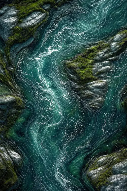
Advected river textures

1. Advected river textures

By Tim Burrell, Dirk Arnold and Stephen Brooks*

We present a new method for the realistic real-time simulation of rivers. Our solution includes a 2D fluid solver that simulates the flow of a river's surface, an efficient method for adaptively computing 3D flow information and an animated 3D procedural wave texture that is advected through the fluid via advection particles in order to mimic the highly detailed fluid surfaces that are characteristic of rivers. Our technique that couples animated texture advection with a pseudo-3D fluid simulation produces stable results that are representative of large-scale real-world rivers and suitable for use in real-time applications. Our system surpasses prior work on real-time river rendering both with regards to efficiency and visual quality, which we establish through the rendering of rivers tens of kilometers long.
Copyright © 2009 John Wiley & Sons, Ltd.

Received: 23 March 2009; Accepted: 24 March 2009

KEY WORDS: water; texture advection; adaptive simulation; rivers; Navier–Stokes equations

A grayscale image showing a highly detailed, textured surface of a river, likely representing the fluid surface simulation described in the paper. The texture is complex and appears to be composed of many small, interconnected elements, possibly representing water molecules or a procedural texture.

1.1. Introduction

Real-time fluid simulation is a challenging problem in which “no single method (exists) that can capture all the subtle effects of water”¹. Our work specifically focuses on real-time river rendering which is problematic for several reasons: the arbitrary 3D terrain geometry of the riverbed must be taken into account, rivers often include situations with both shallow and deep water, even slow moving rivers have highly detailed dynamic geometries, and rivers are generally very large, stretching many kilometers. Rendering large scale river flows for real-time applications is therefore difficult because of the complexity involved in generating a fluid surface that is both detailed enough to be visually realistic and efficient enough to be interactive.

Through experimentation, we have come to believe that in order to realistically simulate and render a river it requires either a full 3D free-surface solver, or a hybrid technique that couples a lower resolution fluid solver to a higher detail fluid surface construction method. Current techniques do not satisfy all these requirements. Existing real-time fluid techniques are either too computationally expensive or do not exhibit large-scale visual properties required for a river. Given these constraints, the goal

of our method is to approximate as much detail as possible while remaining efficient enough for interactive applications. We have also adopted the additional requirement that the method should be suitable for coupling with a rigid-body physics engine allowing 3D objects in the scene to interact with the river's surface. Specifically, we achieve the following: detailed fluid surface construction that responds appropriately to the underlying 3D terrain, simulation of the surface detail of real rivers, above real-time frame rates on commodity hardware, and an algorithm designed with rigid-body coupling in mind. To realize these goals we incorporate a 2D Navier–Stokes solver for its stability, efficiency, and accuracy, that is informed by 3D information gleaned from a series of Hydrostatic Pressure (HSP) columns. We do not use HSP columns alone since it is not a suitable approach for large-scale river representations as it cannot capture detailed effects². We then couple the results of our pseudo-3D Navier–Stokes–HSP fluid solver with a texture advection method in order to derive highly detailed river surfaces. Example renderings running at 60–120 frames per second (85 on average) can be found in Figure 1.

1.2. Previous Work

Many techniques have been developed for different types of fluid simulations including deep water, shallow water, and enclosed volumes of water. Other work has looked at the interplay between fluids and rigid bodies³ and the simulation of hydraulic erosion^4,5. Even phenomena such

*Correspondence to: S. Brooks, 6050 University Avenue, Faculty of Computer Science, Dalhousie University, Halifax, Nova Scotia, Canada, B3H 1W5, Canada.
E-mail: sbrooks@cs.dal.ca

Figure 1: Three side-by-side screenshots of a real-time river rendering. The river is depicted with a blue, slightly translucent surface flowing over a green, textured terrain. The water surface shows subtle ripples and reflections, giving it a realistic appearance.

Figure 1. Real-time river renderings running at 60–120 frames per second on a single core.

as smoke, foam, sand, and clouds have been simulated with fluid dynamics^6–10. Common to all these techniques are a few underlying approaches that range from solving differential equations to methods that simulate water at the particle level.

The most common approach for real-time simulation are Navier–Stokes based solvers. Early work by Chen et al.¹¹ proposed a method for real-time Navier–Stokes; however, the system suffers from instability issues and only operates on limited size volumes of water. Stam's¹² groundbreaking work later outlined techniques for stable advection. Thon and Ghazanfarpour¹³ simplify the problem for rivers by using a 2D Navier–Stokes solver to drive Perlin Noise functions¹⁴ along streaklines. However, their system does not incorporate 3D flow information and produces animations with a procedural appearance lacking key visual features found in rivers. Neyret and Praizelin¹⁵ proposed a simpler model for streams using a two-dimensional Laplace equation, but only produce schematic 2D animations. In recent work, Lee and Sullivan¹⁶ present a method for efficiently computing shallow water equations but only at the expense of stability and they are unable to simulate volumes of fluid at the river scale. To date, real-time free-surface 3D solvers remain unfeasible for large volumes of fluid.

Particle systems instead coarsely model the interaction between individual water molecules^17,18. SPH

methods retain conservation of mass and can represent free-form surfaces and splashing¹⁹. However, such methods are limited by the number of particles that can be used in real-time. In 2003, Müller et al.²⁰ achieve interactive rates with 5000 particles. Clavet et al.²¹ simulate 1000 particles at 10 fps while offering two-way arbitrary object to fluid coupling. Kipfer and Westermann²² simulate rivers using SPH at interactive rates with 3000 particles, though we argue that the fluid does not achieve a truly realistic river surface. In recent years commercial GPU based solutions have appeared that can handle roughly 100,000 particles but even this is insufficient to simulate a river with fine grained detail. Realistic rivers would require perhaps tens to hundreds of millions of particles which is simply not feasible at this time. Though we note SPH has successfully been used offline to create stunning simulations^23,24.

The Wave Particles method by Cem Yuksel, et al.²⁵ is a 2D method that uses deviation functions to perturb a surface heightfield based on interactions with rigid bodies. However, the method does not provide two way fluid-to-fluid and fluid-to-object coupling which means it would still require an underlying fluid simulation. Cords²⁶ later tied wave particles to a 2D Navier–Stokes simulation which yields an enclosed, small body water system. However, it is unable to simulate river-scale systems in real-time and does not take into account the 3D terrain and flow.

Hydrostatic Pressure (HSP) columns presented by Kass and Miller²⁷ and extended to 3D by Mould and Yang²⁸ form a system of columns and pipes that move water based on the laws of hydrostatics. Several simulators incorporate HSP solvers as it is one of the few techniques that is efficient enough to produce a large-scale fluid simulation in real-time. Holmberg and Wunsch² use an HSP based system to represent a very small river section. Their aim was more to generate splashing based on interactions between fluid and terrain than large-scale rivers or a detailed surface representation. Maes et al.¹ later used HSPs and a particle system to model both a river fluid surface and splashing effects. But the method is unstable if time deltas become too large, and does not achieve real-time frame rates even with extensive GPU optimization. HSPs are also “not capable of simulating certain situations such as vortices. A second problem arises from the fact that turbulence is a feature of flow and not of the fluid at rest. This means that . . . the equations generated for flow are incomplete and ignore many of the visible characteristics of water such as viscous shear stresses.”² We therefore do not use HSP columns directly, but use them to inform our NS solver and method of texture advection.

Figure 2: A 3D visualization of a partial HSP grid within a riverbed. The riverbed is shown as a brown, textured surface. Above it, a grid of blue, semi-transparent rectangular columns is visible, representing the HSP columns. The columns are arranged in a regular pattern, and their heights vary, indicating the fluid surface level.

Figure 2. Partial 3D HSP grid visualized within a riverbed.

Other work has employed statistical or procedural fluid simulation. Fournier and Reeves²⁹ pioneering work on deep-water simulation uses a mix of Gerstner waves and Biesel swell models. Work on statistical wave generation by Perlin and Hoffert³⁰ influenced a series of approaches, including Tessendorf’s^31,32 ocean simulators which build on earlier work by Mastin et al.³³. Mitchell³⁴ uses Tessendorf’s technique to great effect, as well as integrating a shallow water solver and object to fluid coupling. The methods in this area are computationally inexpensive but are not directly suited for simulating rivers because the interaction with terrain geometry cannot be easily modeled. Another interesting procedural method is Gerstner waves, which has been used for the realistic rendering of choppy and rapid river water³⁵. But with this method one must explicitly define the parameters of the Gerstner functions and setting these parameters for a series of Gerstner waves is very much an artistic endeavor. Shi et al.³⁶ use a statistical (FFT) procedural approach to generating a fluid surface. However, this work is focused on dynamic fluid routing rather than the fluid representation itself.

Texture advection^12,37 transports colour based on a simulation or function. For our purposes we recast texture advection moving surface waves along a river as dictated by our fluid simulation. Kwatra et al.³⁸ recently tied texture synthesis to a full 3D NS solver. However, as they were not concerned with real-time performance, their technique is not immediately applicable to our problem domain. Their system required up to 200 seconds per frame in order to render a small volume of fluid and it can be argued that they remain somewhat artificial and procedural in appearance.

1.2.1. Real-Time River Simulation

Our hybrid approach to river simulation incorporates 2D Navier–Stokes, HSPs and texture advection in order to achieve the final result. We drive the simulation with

2D Navier–Stokes for its efficiency and stability. This is augmented with the output from HSP columns in order to integrate 3D flow information while still retaining the efficiency of a 2D based fluid simulation. Texture advection is then used to add surface detail to the fluid volume.

1.2.2. 2D Navier–Stokes Simulation

2D Navier–Stokes will provide fluid flow velocity information for the simulation. In our discussion we focus primarily on the relationship between the results of the NS solver, how they apply to the Hydrostatic Pressure Columns, how they are used during the Texture Advection phase and how we achieve a constant flow by applying impulses to the Navier–Stokes velocity field.

The NS solver itself is based on the work of Stam³⁹ which uses a grid of cells where each cell has a velocity and pressure value associated with it. The initial state of the grid is a zero state where all grid cells have zero for both velocity and density. By solving the Navier–Stokes equations the solver modifies the velocities and densities of all cells in the system with the output of one step becoming input of the next.

The simulation represents the fluid on a regular grid $\mathbf{x} = (x, y)$ with time $t$ . The fluid itself is represented as a velocity field, $\mathbf{u} = (\mathbf{x}, t)$ , and a scalar pressure field, $p(\mathbf{x}, t)$ . The equations are then:

$\begin{aligned} \frac{\partial \mathbf{u}}{\partial t} &= -(\mathbf{u} \cdot \nabla) \mathbf{u} - \frac{1}{\rho} \nabla p + \nu \nabla^2 \mathbf{u} + \mathbf{F} + \mathbf{H} \\ \nabla \cdot \mathbf{u} &= 0 \end{aligned} \quad (1)$

where $\rho$ is the fluid density, $\nu$ is the kinematic viscosity of the fluid, $\mathbf{F} = (f_x, f_y)$ are the external forces acting on the fluid and $\mathbf{H}(\mathbf{x}, y)$ is a function that returns HSP pressure information. In addition we use standard Neumann boundary conditions for the river banks. These equations express the standard components of any fluid simulation: advection, pressure gradient, diffusion, and external forces. The reader is referred to Stam^12,29 for further discussion of the Helmholtz–Hodge decomposition.

1.2.3. Hydrostatic Pressure Columns

The 2D NS simulation gives the fluid surface the ability to appropriately interact with river banks and obstacles, but lacks the ability to simulate inter-fluidic shear stresses and 3D interactions with the terrain. We therefore augment the 2D NS simulation with Hydrostatic Pressure (HSP) columns²⁷ which provide pseudo-3D fluid flow in addition to pressure information. Our method couples the HSPs with the NS solver in order to affect the NS velocity and pressure fields based on the 3D pressure information from the HSP grid.

An HSP grid is constructed and used to compute pressure values at each grid cell in the fluid volume, using the laws of hydrostatics. The fluid volume is discretized into small columns which are further split vertically into cells (see Figure 2). Each cell's pressure is computed based on the pressure of neighboring cells. The laws of hydrostatics dictate that fluid will attempt to equalize its pressure which is used to determine the rate that fluid flows from one cell to another.

The movement of fluid between cells is accomplished by connecting the cells to their neighbors via a series of pipes. When there are multiple cells touching one side of a cell, a pipe is created for each overlapping cell. This pipe's size, called the pipe cross-section, is determined by the amount of overlap:

$C_{\text{pipe}} = (h_{\text{top}} - h_{\text{bottom}}) \times d \quad (2)$

where $d$ is the length of the pipe (equal to the grid spacing) and the tops and bottoms of the pipes are the min and max of the tops and bottoms of the cells into which the pipe flows:

$h_{\text{top}} = \min(a_1, a_2), h_{\text{bottom}} = \max(b_1, b_2) \quad (3)$

where $a_n$ is the height of cell $n$ and $b_n$ is its base.

Figure 3: A 4-step diagram illustrating the fluid flow simulation process. Step 1 shows a 3x3 grid of cells with the top-left cell highlighted in blue and containing a small blue arrow pointing right. Step 2 shows the top-left cell and its right neighbor highlighted in blue, with arrows pointing right. Step 3 shows the top-left cell, its right neighbor, and the cell below the top-left cell highlighted in blue, with arrows pointing right. Step 4 shows the top-left cell, its right neighbor, the cell below the top-left cell, and the cell below the right neighbor highlighted in blue, with arrows pointing right. The other cells in the grid are brown.

Figure 3. In step 1, the top-left cell has its velocity calculated and this information is saved as the flow hint. In step 2, cells adjacent to the first cell are computed which are again saved as flow hints. Once all cells have flow hints (step 4) the system is primed and constant flow is achieved through the application of impulses.

The pipe cross sections are re-computed at every simulation step since they change as the pressures in the cells change. However, before calculating any volume transfer we need to first compute the pressure of each cell as follows:

$p = h_{ij}\rho g + p_0 + p_{ij} \quad (4)$

such that $h_{ij}$ is the height of column at position $(i, j)$ , $\rho$ is the density of the fluid, $g$ is the force of gravity, $p_0$ is the atmospheric pressure and $p_{ij}$ is an external pressure being exerted on the column at position $(i, j)$ due to rigid body interaction or an impact on the fluid surface.

Once the column pressures are computed and the pipe cross sections are determined, the next step is to calculate the flow velocity and resultant flow volume through the pipes using the pressure differences between cells. The velocity through any given pipe is given as:

$n = f\mathbf{u}_0 + \Delta t \frac{(p_{\text{head}} - p_{\text{tail}})}{\rho} \quad (5)$

where $f$ is a friction coefficient, $\mathbf{u}_0$ is the flow velocity from the previous time step, $\Delta t$ is the time delta, $p_{\text{head}}$ is the pressure of the cell at the head of the pipe, $p_{\text{tail}}$ is the pressure of the tail cell and $\rho$ is the density of the liquid. The volume of fluid that passes through a pipe is defined as:

$v = \Delta t \times n \times c_{\text{pipe}} \quad (6)$

where $c_{\text{pipe}}$ is the cross sectional area of the pipe.

During the simulation the fluid transfers may cause one or more cells to have a negative volume. To compensate for this, the total outflows from each cell are first calculated, then each cell is checked to see if it will contain a negative volume. If a cell would contain negative volume, all pipes flowing out of the cell are scaled back by an amount equal to a percentage of the total cell outflow and the negative amount of fluid that the cell would contain. For example, if a 10% overflow has occurred, each outflowing pipe is scaled back by 10% of the amount that flowed through it, as opposed to 10% of the total overflow. This process continues until all cells contain a non-negative amount of fluid.

Since the HSP columns are not the primary simulation they can be run under precisely controlled conditions such that explosions do not occur. We only re-calculate the columns whenever the fluid volume's path requires updating; in our test application this is only done once at program startup. Because of this HSP stability is not an issue. Furthermore, in a large fluid body such as a river, our experiments showed that the HSP pressure field did not vary significantly over time. We therefore only run the HSP simulation once to obtain the general pattern of flow and vary the 3D pressure information over time via random fluctuations. We modulate pressure information in order to approximate the subtle pressure changes that would occur if the simulation was re-computed at every time-step:

$\bar{p}_{ij} = p_{ij} \text{rand}(r_{\min}, r_{\max}) + p_{ij} \quad (7)$

where $p_{ij}$ is the pressure at column $(i, j)$ , and $\text{rand}()$ returns a random value from $r_{\min} = -0.05$ to $r_{\max} = 0.05$ , such that the final value will be $\pm 5\%$ of $p_{ij}$ . It should be stressed that this step is optional since running simulations with and without the random variance produces results that look only slightly different. The main effect is due to the 3D pressure information.

1.2.4. Bootstrapping the Hydrostatic Pressure Columns

It is difficult to produce large-scale constant flows that rivers exhibit with HSPs alone. Because of this we bootstrap the HSP solver with external constant flow information. We adapt our NS solver to achieve a constant flow and provide the HSP simulation its flow information from a single run of a strictly 2D Navier-Stokes flow simulation. This initial simulation is the first step in the simulation.

The HSP computations are dependent on the velocity in the previous time step. Therefore in order to generate an HSP pressure map we simply substitute the initial phase of NS velocity output into the velocity component, $u_0$ , of the HSP velocity update equation. This bootstrapping procedure only provides the HSP simulation with the initial flow rate and direction of each hydrostatic pressure column cell. Once these values are input into the HSP solver, the resulting 3D flow information is entirely based on the 3D terrain underneath and inside the fluid volume.

After the initial Navier-Stokes system is solved, and the results have been provided as input to the HSP solver, the resultant pressure grid is used, in turn, to influence the augmented 2D Navier-Stokes solver with the 3D pressure data. And since rivers are basically static with regards to their flow path we can simply pre-compute and store the HSP grid prior to simulation. The algorithm completes a single HSP update in approximately 3–5 seconds with a column depth of three cells.

1.2.5. Impulse Driven NS

There remains an issue that arises when simulating a large body of fluid. Specifically, the simulation must be primed with large areas of off camera fluid in order to generate the necessary momentum inherent in an open system. Moreover, it is not possible to accurately simulate a river by simply placing a source at one end and a sink at the other. In order to achieve the desired flow rates, the source and sinks would require such large pressure values that major artifacts would emerge.

Our solution is related to a technique used in rigid-body physics engines: the application of impulses. We will apply small impulses to each cell in order to maintain flow. There are, however, issues with this approach that must be addressed. For example, in what direction should impulses be applied, particularly if the local flow is in opposition to the mean direction of the river? Another issue is what the initial state of the river should be and how are the first rounds of impulses to be applied?

Before applying the impulses an initial state must be computed so that we know which direction and with what magnitude the impulses should be applied. We refer to this process as priming the flow which is depicted in Figure 3. First, an impulse field is propagated across the simulation grid over a number of steps starting with an initial impulse hint from the user at one edge of the river which dictates the basic direction of the river. The first time step causes the impulses to be applied as the fluid is solved. At any cell where the velocity is not zero, that velocity vector is normalized and saved as the flow hint for that cell. In the next time step impulses are applied to the initial cells given by the user and those cells already affected by the simulation. The algorithm sweeps across the river in successive time-steps from the user specified source location. This is repeated until all cells have a flow hint associated with them. In the second phase of the flow priming procedure the simulation is run with flow hinting enabled until one “advection particle” is able to travel the length of the river.

Equipped with the flow hinting field and a primed fluid volume we begin adding impulses to each cell in the simulation as it runs. As we do so we need to ensure the simulation stability is not compromised, complex flows can still be visualized and the overall flow does not exhibit incorrect flow behavior such as a river reversing its direction. To accomplish this, the magnitude of the impulse added to a cell is made proportional to the cell’s velocity in relation to the desired flow volume. For example, if two cells had the same flow hint, with one having a velocity of 1.0 units of flow and the other 0.5, the faster moving cell would be affected twice as much as the slower moving cell during the application of the impulse. In this way, the impulse application scales linearly and the ratio between one cell and another does not change after the impulses are applied (given equal circumstances the difference in rate of flow between once cell and the next will have the same ratio after the impulse application).

The direction of the impulse is then modified based on the deviation between the flow hint vector and the current velocity vector. In order to calculate the cell's directional deviance, $d$ , from the flow hint we use the standard geometric angle difference:

$d = \text{abs}(\text{rad2deg}(\text{atan2}(u.y, u.x) - \text{atan2}(f.y, f.x))) \quad (8)$

where $v$ is the cell's velocity, and $f$ is the flow hint. We then check if $d$ is greater than or equal to a cutoff deviance value and if so we calculate an impulse for the cell using the cell's current velocity vector and the cell's previously calculated flow hinting value. From our experiments, we found values around $15^\circ$ to be an effective cutoff value that works across different simulations. With numbers significantly less than $15^\circ$ the visual diversity of the simulation is impacted as the ability for opposing flows or fluidic shearing is overly constrained. Conversely, as the value is relaxed the general flow of the river becomes too variable and less visually realistic. A compromise between flow diversity and the general river flow is therefore necessary.

We must also incorporate the data provided by the hydrostatic pressure columns, which augments our simulation with 3D information. For this we simply scale the impulse velocity by the pressure value returned from the cell's associated HSP column:

$l_{ij} = \|\mathbf{u}_{ij}\| \frac{p_{ij}}{P} z \quad (9)$

where $l_{ij}$ is the new impulse magnitude for cell at index $(i, j)$ , $\mathbf{u}_{ij}$ is the cell's velocity, $p$ is the HSP pressure, $P$ is the maximum pressure the HSP simulation can contain and $z$ is a user defined value such that $0 \leq z < \infty$ . By changing $z$ with a slider one can influence how much the HSP information affects the simulation. However, for all our simulations we keep $z$ at 1.0. The sum of all these modified impulses is then equal to the desired flow velocity.

For effect, we can also add other factors as well, such as a small random variance to either the impulse direction or velocity, or to how much the HSP columns affect the

simulation. Such variances will result in a more, or less turbulent river. It is also possible to apply a maximum and/or minimum flow rate check in order to match the river flow to a desired look. In our examples, the random variance factor is set to be plus or minus 1%, and maximum and minimum flow speeds to be no more (or less) than 200 times greater than or less than the mean flow speed.

It should also be noted that the flow speed of the river itself should be set in accordance to the grid cell size of the river in order to maintain grid size independent flow rates. For example, if the desired flow rate is 1.3 meters per second and the cell width is 1.0 unit, the flow rate should be set to one half the value of the same flow rate on a grid with a cell width of 2.0 units.

1.2.6. River Surface Advection

We have defined a highly efficient pseudo-3D fluid simulator, however, this alone is not sufficient to derive the highly detailed surface deformations found in real rivers, we therefore incorporate texture advection of animated ocean waves. We first discuss the formation of the animated wave texture itself which is generated procedurally while the simulation runs. We experimented with a number of techniques including random noise and Gerstner Waves³⁵. But, we chose to adapt the method presented by Mitchell³⁴ which is derived from Tessendorf's³¹ FFT method for Ocean waves. This approach computes large quantities of realistic waves at a low cost. The fluid surface is defined as a heightfield where the height of any grid cell, $\mathbf{x}$ at a given point in time, $t$ , is:

$h(\mathbf{X}, t) = \sum_{\mathbf{k}} H(\mathbf{k}) e^{i(\mathbf{k} \cdot \mathbf{x} - \omega(\mathbf{k})t)} \quad (10)$

where $h$ is the height field, $\omega$ is the angular wave frequency, $H(\mathbf{k})$ contains amplitude and phase information, $\mathbf{k}$ is a 2D vector such that $k_x = 2\pi n / L_x$ , $k_y = 2\pi m / L_y$ and $(n, m)$ are integers with bounds $-N/2 \leq n < N/2$ and $-M/2 \leq m < M/2$ .

However, procedural techniques are not intended to simulate a fluid volume and so the static wave fronts must be transported such that they have the appearance of moving with the river. One can think of moving a carpet around a curved track. But our situation is more complex because we must simultaneously move every section of the carpet in a different direction and at a different speed. The principle behind texture advection is to transport or morph one or more textures over time based on a series of input parameters (see Figure 4). In our case, we use velocity and pressure information from the pseudo-3D fluid simulator to advect the wave texture using what we will call river particles. These particles are propagated through the fluid using the results of the velocity and pressure information from the NS simulation. A river particle is an encapsulation of a mathematical deviation function that describes how a particular section (texel) of a texture is to be propagated through space and time.

Figure 4: Texture advection. The left image shows a 6x6 grid of colored squares (red, magenta, blue, cyan, green, yellow) with black arrows representing velocity components and small black circles representing river particles. The right image shows the resulting texture after advection, where the particles have moved and the colors are now a mix of the original colors, representing the advected texture.

Figure 4. Texture advection. Arrows (left) represent velocity components of the fluid simulator and circles represent river particles. The resultant image after being advected is shown right.

The task of advecting the wave texture is similar to the procedure that the Navier–Stokes advection solver uses. A back-trace is performed on each point in the volumetric grid to its source location in the previous time step:

$p(\mathbf{x}, t + \Delta t) = p(\mathbf{x} - \mathbf{u}(\mathbf{x}, t)\Delta t, t) \quad (11)$

where, $\mathbf{u}(\mathbf{x}, t)$ is the particle's current position, and $-\mathbf{u}(\mathbf{x}, t)\Delta t$ is the vector that we use to translate the particle back through time by the amount specified in $\Delta t$ . Note that, as with the NS advection, this step will likely place the particle somewhere in between four grid cells, so we perform bilinear interpolation from the four neighboring grid cells to compute the end result.

In addition, each river particle has the following properties: location in the input textures, birth location, age, current location in the river, and age at death. An advection particle pertains to a specific location in the input textures which does not change. For our application we use an animated texture comprised of a number of frames of individual textures. The location in the input textures refers to the same location in each texture, where one texture is a single frame of the texture animation.

This particle is then introduced into the fluid simulation and affected by the fluid simulation's velocity and pressure fields so that it moves through the river. As it moves it affects the resultant wave texture

by adding its value from the input textures to the output texture. Each location in the output texture can be seen as the average of all particles currently occupying that location:

$O_{xy} = \frac{\sum_{i=0}^n f(p_i)}{n+1} \quad (12)$

where $f(p_i)$ is a function that returns the value of the particle's combined input textures. We use a texture resolution equal to the grid resolution at its highest level of detail setting so that the resulting surface is no more or less detailed than the geometry itself. The number of advection particles varies over time as they spawn, however, the initial state matches the number of advection particles with the grid resolution of the advection texture.

Particles are spawned at specific times and have limited lifespans. They also do not travel infinitely far from their birth location because after traveling a certain distance they become completely un-grouped from their neighbors and start to resemble noise rather than wave fronts. In addition, the particle's age determines how strongly the output texture is affected by that particle. If a particle was recently spawned it fades in and as a particle nears its time of death it fades out, thus removing visual popping artifacts. The particle's current location has a similar impact, in that the farther a particle strays from its birth location the less of an impact it has on the final wave summation. We therefore define the particle update function to be:

$f(P) = \frac{a_c - a_b + \frac{\|l_c - l_b\|}{L}}{2} \quad (13)$

where $a_c$ is the particle's current age, $a_b$ its birth time, while $l_c$ and $l_b$ denote the particle's current and birth locations. $A$ is a constant defining the average age of a particle and $L$ determines the maximum distance a particle can be from its birth location without being transparent. For all our simulations we set $A$ to be 1.5 seconds and $L$ to be 5% of the total length of the river.

The average lifespan, $A$ , of the particles can be adjusted depending on how turbulent and quickly the river is moving. Our system provides a graphical particle display that assists in the adjustment of this value, as seen in Figure 5. By representing each particle as a color determined by its birth location it is easy to see how far the particles remain traveling in groups of similar color. We note that there is significant leeway in choosing good settings for these parameters; finding a single optimum setting for these constants is not required since the system is not overly sensitive to the tuning of this parameter. Moreover, we use a pseudo-random function with values in the range of (0.5, 2.0) to scale each particle's life span with respect to the average, $A$ . The aim being to avoid situations in which many particles are dying or spawning simultaneously.

Figure 5: Visualization of advection particles. The image shows a dense field of small, colorful particles (pink, purple, and green) moving across a green, textured terrain. The particles are concentrated in a central area, suggesting a flow or advection process.

Figure 5. Visualization of advection particles. The number of particles has been reduced to improve clarity.

In the initial bootstrapping phase, we first assign an advection particle to every cell in the grid. We then run the simulation until all initial advection particles have died and respawned at least once, thereby reaching a stable state. In practice this requires a few seconds of

computation on 10 km river, but can be pre-computed and stored. When no particle remains in a cell, a new one is faded into existence with its birth location set to an average of its neighbors. This removes the situation where a section of a river becomes empty and also eliminates any visual popping that might occur at the introduction of new particles. As can be seen in Figure 5, particles travel together in loose groupings where particles instantiated in similar locations remain near to one another. Yet features such as vortices and directionally opposing fluid flows can still be seen.

1.3. Results

Our real-time method for simulating and rendering rivers is visually more convincing than existing methods and runs at far higher frame rates. Minute details in the river flow can be seen as a result of complex interactions between fluid and terrain and the fluid with itself. These complex interactions are a direct result of combining HSP columns with a 2D Navier-Stokes solver.

The texture advection step produces highly detailed fluid surfaces in which the water interacts with the underlying terrain in ways typically reserved for the fully 3D fluid solvers. Water can be seen speeding up over shallow sections and slowing down over deep sections, as well as becoming turbulent in areas with large underwater obstacles, getting caught in nooks and eddies and flows around bends. This can be partially seen in Figures 1 and 7 clearly seen in the provided video (available online at www.interscience.wiley.com/journal/cav). Figure 6 shows a comparison between the simulation running with the HSP columns turned on and off. In the case with HSP columns turned off the simulation is purely using the 2D Navier–Stokes for simulation results, and any terrain to fluid interactions are only at the shoreline and at the very surface of the fluid.

Figure 6: Comparison of hydrostatic pressure columns. The top row shows two side-by-side views of a river flow on a textured terrain. The left view shows the flow with hydrostatic pressure columns disabled, appearing smoother. The right view shows the flow with hydrostatic pressure columns enabled, showing more detailed, turbulent features. The bottom view shows the underlying terrain, which is a green, textured surface with a central dark area.

Figure 6. Comparison with the hydrostatic pressure columns disabled (left) and enabled (right). Underlying terrain shown below.

A 3D rendered image of a river flowing through a green, hilly landscape. The river is dark blue and shows some eddies and bends. The terrain is covered in green vegetation.

Figure 7. Real-time rendering of long river section.

Level of Detail provides notable performance improvements as can be seen in Table 1. Even the modest LOD optimizations we have implemented make a significant difference to the frame rate and to the number of polygons rasterized per second. All screenshots and timings were produced on an off-the-shelf dual-core Athlon XP 3800+ computer with an nVidia 8600GT graphics card and 4GB RAM. However, the code has not been parallelized or GPU optimized, meaning that only one of the two cores on the CPU has been directly used. Most of example river beds used in this paper have been imported from DEM files of real rivers.

Level of detail	FPS	Poly's per second
Fully disabled	63	61 million
Texture advection only	74	71 million
Navier–Stokes only	111	107 million
Fully enabled	120	115 million

Table 1. Comparison of the simulation running with different types of LOD enabled

1.4. Conclusion

We have developed an efficient approach to rendering large-scale fluid flows over arbitrary terrains with a relatively high level of realism. By combining an impulse driven 2D Navier–Stokes simulation with multi-tier hydrostatic pressure columns we have created a low computational-cost fluid solver that provides sufficient 3D information to simulate a river in real-time. We then employ procedural wave generation to produce an animated texture which is advected through the fluid simulation. This produces a highly detailed fluid surface representation that exhibits many of the visual elements that are characteristic of rivers. Our technique is applicable to real-time and interactive simulation scenarios and has been designed with rigid-body physics objects in mind. We feel that this work is therefore a major step forward in the area of real-time river rendering for interactive applications.

1.5. Future Work

This work affords many avenues of interesting further research. Our current implementation does not simulate non-planar fluid surfaces, though the method could be augmented to do so since pressure information is available directly from the simulation at every cell. This system could also easily integrate with a foam/particulate engine for waterfalls and large sprays. Other work could also examine alternate procedural texture/wave generation methods. Another enhancement would be the addition of two-way rigid-body to fluid interactions. As previously noted, we designed the system with this in mind by building the API from the ground up to allow individual scene objects to have full access to the fluid simulator's velocity and advection information.

Further work could explore improvements to Level of Detail rendering for rivers. Our system currently uses only basic geometry LOD on the terrain and no geometric LOD on the river surface itself. Although the river sections are split into LOD patches, this is only for the purpose of changing detail levels within the fluid simulation algorithm. We believe that adding a sophisticated geometry LOD algorithm would allow the simulation and rendering to operate at an even higher frame rate.

1.6. ACKNOWLEDGEMENTS

This work has been funded by NSERC and the Canadian Foundation for Innovation.

1.7. References

1. Maes MM, Fujimoto T, Chiba N. Efficient animation of water flow on irregular terrains. In GRAPHITE '06, 2006; 107–115.
2. Holmberg N, Wunsche B. Efficient modeling and rendering of turbulent water over natural terrain. GRAPHITE '04, 2004; 15–22.
3. Carlson M, Mucha PJ, Turk G. Rigid fluid: animating the interplay between rigid bodies and fluid. ACM Transactions on Graphics (Proceedings of SIGGRAPH) 2004; 23: 377–384.
4. Mei X, Decaudin P, Hu B. Fast hydraulic erosion simulation and visualization on GPU. Pacific Conference on Computer Graphics and Applications, 2007; 47–56.
5. Stava O, Benes B, Brisbin M, Krivanek J. Interactive terrain modeling using hydraulic erosion. ACM SIGGRAPH/Eurographics Symposium on Computer Animation, 2008; 30–39.
6. Foster N, Metaxas D. Modeling the motion of a hot, turbulent gas. In Proceedings of SIGGRAPH 97, 1997; 181–188.
7. Fedkiw R, Stam J, Jensen W. Visual simulation of smoke. ACM SIGGRAPH, 2001; 15–22.
8. Takahashi T, Fujii H, Kunimatsu A, Hiwada K, Saito T, Tanaka K, Ueki H. Realistic animation of fluid with splash and foam. Computer Graphic Forum 2003; 22(3): 391–400.
9. Losasso F, Gibou F, Fedkiw R. Simulating water and smoke with an octree data structure. ACM Transactions on Graphics (Proceedings of SIGGRAPH) 2004; 23(3): 457–462.
10. Zhu Y, Bridson R. Animating sand as a fluid. ACM Transactions on Graphics (Proceedings of SIGGRAPH) 2005; 24(3): 965–972.
11. Chen JX, Da Vitoria Lobo N. Toward interactive-rate simulation of fluids with moving obstacles using navier-stokes equations. CVGIP: Graphical Model and Image Processing 1995; 57(2): 107–116.
12. Stam J. Stable fluids. In ACM SIGGRAPH, 1999; 121–128.
13. Thon S, Ghazanfarpour D. A semi-physical model of running waters. Computer Graphic Forum (Proceedings of Eurographics) 2001; 19: 53–59.
14. Perlin K. An image synthesizer. SIGGRAPH Computer Graphics 1985; 19(3): 287–296.
15. Neyret F, Prazelin N. Phenomenological simulation of brooks. In Eurographics Workshop on Computer Animation and Simulation. Springer: Eurographics, 2001; 53–64.
16. Lee R, O'sullivan C. A fast and compact solver for the shallow water equations. Virtual Reality Interactions and Physical Simulation 2007; 1(1): 51–58.
17. Lucy LB. A Numerical approach to testing the fission hypothesis. Astronomical Journal 1977; 82: 1013–1024.
18. Gingold R, Monaghan J. Smoothed Particle Hydrodynamics: Theory and Application to Non-Spherical Stars, 1977; 375–389.
19. O'brien JF, Hodgins JK. Dynamic simulation of splashing fluids. In Computer Animation 1995; 95: 198–205.
20. Müller M, Charypar D, Gross M. Particle based fluid simulation for interactive applications. In Eurographics/ SIGGRAPH Symposium on Computer Animation, 2003; 154–159.
21. Clavet S, Beaudoin P, Y PP. Particle-based viscoelastic fluid simulation. In ACM SIGGRAPH/Eurographics Symposium on Computer Animation, 2005; 219–228.
22. Kipfer P, Westermann R. Realistic and interactive simulation of rivers. In Proceedings of the Graphics Interface, 2006; 41–48.
23. Irving G, Guendelman E, Losasso F, Fedkiw R. Efficient simulation of large bodies of water by coupling two and three dimensional techniques. ACM Transactions on Graphics (Proceedings of SIGGRAPH) 2006; 25(3): 805–811.
24. Losasso F, Taltou J, Kwatra N, Fedkiw R. Two-way coupled SPH and particle level set fluid simulation. IEEE Transactions on Visualization and Computer Graphics 2008; 14(4): 797–804.
25. Yuksel C, House DH, Keyser J. Wave particles. ACM Transactions on Graphics (Proceedings of SIGGRAPH) 2007; 26(3): 1–12.
26. Cords H. Moving with the flow: wave particles in flowing liquids. International Conference in Central Europe on Computer Graphics, Visualization and Computer Vision, 2008.
27. Kass M, Miller G. Rapid, stable fluid dynamics for computer graphics. In Computer Graphics (SIGGRAPH '90 Proceedings) 1990; 24: 49–57.
28. Mould D, Yang Y. Modeling water for computer graphics. Computers & Graphics 1997; 21(6): 801–814.
29. Fournier A, Reeves WT. A simple model of ocean waves. Computer Graphics (Proceedings of SIGGRAPH 86) 1986; 20: 75–84.
30. Perlin K, Hoffert EM. Hypertexture. Computer Graphics (Proceedings of SIGGRAPH) 1989; 23(3): 253–262.
31. Tessendorf J. Simulating ocean water. SIGGRAPH Course Notes, 2001.
32. Tessendorf J. Simulating ocean surfaces. SIGGRAPH Course Notes, 2004.
33. Mastin GA, Watterberg PA, Mareda JF. Fourier synthesis of ocean scenes. IEEE Computer Graphics and Applications 1987; 7(3): 16–23.
34. Mitchell J. Real-time synthesis and rendering of ocean water. Technical Report 2004, Marlboro, MA.
35. Brown S, Collier R. Flooding ice age: the meltdown using wavesynth and point based froth. In ACM SIGGRAPH 2006 Sketches, 2006, 21.
36. Shi S, Xiuzi Ye ZD, Zhang Y. Real-time simulation of large-scale dynamic river water. Simulation Modeling Practice and Theory 2007; 15(6): 635–6646.
37. Neyret F. Advected textures. Proceedings of ACM SIGGRAPH/Eurographics Symposium on Computer Animation, 2003; 147–153.
38. Kwatra V, Adalsteinsson D, Kim T, Kwatra N, Carlson M, Lin MC. Texturing fluids. IEEE Transactions on Visualization and Computer Graphics 2007; 13(5): 939–952.
39. Stam J. Real-time fluid dynamics for games. The Game Developer Conference, 2003.

1.8. Authors' biographies:

A black and white portrait of Tim Burrell, a man with short, light-colored hair, looking directly at the camera with a neutral expression.

Portrait of Tim Burrell

Tim Burrell received a B.Sc. in Computer Science from the University of Calgary in 2006, and M.C.Sc. from Dalhousie University in 2009. His primary research interests include Computer Graphics, Parallel Programming, and Compiler Design/Language Theory.

A color portrait of Stephen Brooks, a man with short brown hair and glasses, wearing a blue and white checkered shirt, smiling at the camera.

Portrait of Stephen Brooks

Stephen Brooks received his Ph.D. from the Computer Laboratory, University of Cambridge, England, in 2004. He is an Associate Professor with the Faculty of Computer Science, Dalhousie University, Halifax, Nova Scotia, Canada. His research interests span the fields of computer graphics and visualization.

A color portrait of Dirk Arnold, a man with short brown hair and glasses, wearing a dark grey shirt, smiling at the camera.

Portrait of Dirk Arnold

Dirk Arnold received the Ph.D. from the Department of Computer Science, University of Dortmund, Germany, in 2001. He is an Associate Professor with the Faculty of Computer Science, Dalhousie University, Halifax, Nova Scotia, Canada. His research interests include evolutionary computation, optimisation, and computer graphics.