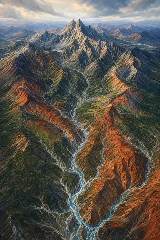
Large Scale Terrain Generation from Tectonic Uplift and Fluvial Erosion

Uplift and faults. Terrains result from the combined action of tectonic uplift of the Earth’s surface and erosion. Collisions between continental plates, as well as subduction of ocean plates under continental ones, cause the continental crust to shorten and thicken. This results in the growth of mountains along the main boundaries between plates. Faults and folds appear in regions where the crust undergoes the highest stress [WBF93].

In geology, the term uplift is used to denote the local speed at which a mountain grows. Because the growth occurs between the series of parallel folds (and faults), considering the uplift as locally uniform between these folds is a valid approximation. The complex landform features found in nature are mainly the result of the interaction between the uplift factor and fluvial erosion, i.e., the action of water forming streams that carve the terrain while it grows.

Fluvial erosion is the erosion of the bedrock material and its transportation downhill by streams. It is caused by the shear stress exerted by running water and the sediment it contains onto the bed of a stream. The interaction between the fluvial erosion and the tectonic uplift has been studied for many years in geology and is usually modeled by the stream power equation [WT99]:

The stream power equation states that the rate of change of surface topography $h(\backslash mathbf\{p\})$ at a position $\backslash mathbf\{p\}$ is controlled by the balance between the surface uplift $u(\backslash mathbf\{p\})$ and the fluvial erosion, which is a function of the local slope $s(\backslash mathbf\{p\})$ and the drainage area $A(\backslash mathbf\{p\})$. The local slope $s(\backslash mathbf\{p\})$ is defined as the surface topographic gradient:

The constants $m$ and $n$ depend on rock strength, climate, and the topology of river networks. While the values of those parameters are poorly understood, the ratio $m/n$ is constrained by the shape of the stream profiles and is thought of being $m/n\; \backslash approx\; 0.5$ [WT99]. As in most geomorphological studies, we use $n\; =\; 1$ and $m\; =\; 0.5$. Moreover, some geological studies attempt to tune these parameters by example [CB14] and a recent survey [Lag14] studies the limit of geological knowledge regarding the parameters of the stream power equation.

The drainage area $A(\backslash mathbf\{p\})$ is the upstream area draining through point $\backslash mathbf\{p\}$, assuming that water flows along the topographic gradient (Figure 3). In our implementation, the terrain is represented by a geometric graph $\backslash mathcal\{G\}$ connecting points sampled over the terrain domain. The drainage area $A(\backslash mathbf\{p\})$ is the area associated to the set of points $\backslash \{\backslash mathbf\{q\}\; \backslash in\; \backslash mathcal\{G\}\backslash \}$ strictly above $\backslash mathbf\{p\}$ such that there exists one path of strictly increasing height starting from $\backslash mathbf\{p\}$ and ending at $\backslash mathbf\{q\}$. The factor $k$ is an erosion constant that depends on many factors, such as lithology (the composition of the soil/bedrock), vegetation, climate, and climate variability.

Note that, when applied at the right temporal and spatial scales (typically between $10^5$ and $10^7$ years and a few tens to hundreds of kilometers), the stream power equation does not only model erosion, but also captures the way a complex relief emerges from a supposedly flat part of the continental crust [How94].

The input to our algorithm (Figure 2) is the uplift map $\backslash mathcal\{U\}$ defining the speed at which the terrain is elevated by tectonics. We define it as a piece-wise uniform distribution of values over the domain $\backslash Omega$. It is given by the user as gray-scales images. The output is a vector-based representation of the terrain resulting from the interaction between the uplift and the fluvial erosion, and in the case of the final high quality rendering, a set of procedural feature elements.

Our algorithm proceeds in two main steps: erosion simulation computed on planar graph $\backslash mathcal\{G\}$ embedding elevation and flow information, called the stream graph, and conversion of this graph into an elevation model $\backslash mathcal\{M\}$ representing the terrain.

Erosion simulation. Starting from the input domain $\backslash Omega$ where the uplift $\backslash mathcal\{U\}\; \backslash neq\; 0$, we initialize the stream-graph $\backslash mathcal\{G\}$ as a random planar graph defined by triangulating uniformly distributed terrain sample points $\backslash mathbf\{p\}\_k$ in $\backslash Omega$. We set the initial elevation of the nodes $h\_k$ of $\backslash mathcal\{G\}$ to zero. We then iterate the stream power equation until we get plausible elevation information (or water flow directions) associated to each node (or arc) of $\backslash mathcal\{G\}$. This is done by iterating the following steps until convergence (Figure 4):

We define the set of directed stream trees $\backslash mathcal\{T\}$ as follows. For each node $N\_k$, considering that water only flows from $N\_k$ to its neighbor $N\_l$ of the lowest elevation $N\_l$, which we call the receiver of $N\_k$, we connect $N\_k$ to $N\_l$ by an arc (a directed edge). Since these connections cannot create loops, they result in a set of trees that are oriented from leaves (i.e., the nodes that are not receivers for any other node) to the root nodes (i.e., lakes or outflows from the $\backslash Omega$). By construction, the set $\backslash mathcal\{T\}$ covers $\backslash mathcal\{G\}$, in the sense that all the nodes of $\backslash mathcal\{G\}$ are included, although only a subset of the edges from $\backslash mathcal\{G\}$ is represented by arcs in $\backslash mathcal\{T\}$. Note that during the first iteration, when all nodes are of height zero, no arc is created and each node is initialized by a tree with only a root node.

The stream trees $\backslash mathcal\{T\}$ cannot be used directly to simulate water flow over $\backslash Omega$ because these trees are not connected, and the water would stop at internal root nodes that represent lakes. While a solution for connecting lakes to other nodes was proposed as an optional step of the main $O(N)$ algorithm in [BW13], adding this step leads to a complexity of $O(N\backslash sqrt\{N\})$, where $N$ denotes the number of nodes. We describe below a more efficient solution that performs lakes connection in $O(N\; +\; M\; \backslash log(M))$ where $M\; \backslash ll\; N$ is the number of lakes.

Abstraction of the lake flows. Lakes are located at the root nodes $N\_l\; \backslash in\; \backslash mathcal\{T\}$ that are not on the boundary of $\backslash Omega$. We assign the unique identifier $L(N\_k)\; =\; l$ to $N\_l$ and to all the nodes $n\_k$ belonging to the same tree (i.e., in the drainage area of $N\_l$), to represent water passing through these nodes and flowing to the lake $n\_l$. As the water level rises, some of these upper nodes will be absorbed by the lake before water overflows.

Our goal is to model overflow between these different lakes down to the river mouths that connect the graph to the outside. We create a directed super graph of lakes $G\_L$, where each group of nodes in $\backslash mathcal\{G\}$ with the same identifier $L(N)\; =\; l$ is represented by a single node $N\_l$. Extra nodes are created to represent river mouths (root nodes at the border of $\backslash Omega$) and their stream tree.

We call a pass the lowest pair $(\backslash mathcal\{X\},\; \backslash mathcal\{Y\})\; \backslash in\; \backslash mathcal\{G\}$ of two neighboring nodes $\backslash mathcal\{X\}$ and $\backslash mathcal\{Y\}$ belonging to different lakes $L(\backslash mathcal\{X\})\; \backslash neq\; L(\backslash mathcal\{Y\})$. Formally, a pass $(N\_i,\; N\_j)$ between two lakes identified by $l\_0$ and $l\_1$ needs the height of its nodes to satisfies: $\backslash forall\; k,\; l$ such that $L(X\_k)\; =\; l\_0$ and $L(X\_l)\; =\; l\_1$, $\backslash max(h\_i,\; h\_j)\; \backslash leq\; \backslash max(h\_k,\; h\_l)$. This $\backslash max(h\_i,\; h\_j)$ is called the pass height. The pass is a connection between both lakes; it corresponds to a saddle point in terms of elevation in the stream graph $\backslash mathcal\{G\}$. Lakes are connected by adding an arc $(L(\backslash mathcal\{X\}),\; L(\backslash mathcal\{Y\}))$ for each pass $(\backslash mathcal\{X\},\; \backslash mathcal\{Y\})$ as shown in Figure 5. Because it is not yet clear in which direction the water will flow, we add two arcs in opposite directions. The opposite arc $(j,\; i)$ between the two lakes $i$ and $j$ has the same pass tuple $(\backslash mathcal\{X\},\; \backslash mathcal\{Y\})$. These arcs represent the two possible flow directions.

Extraction of the lake connections. In the next step we compute a set of trees $T\_L$ covering $G\_L$. This step is analogous to the stream

tree calculation from Section 4.2, but this time we model the flow between lakes. Unfortunately, this cannot be done in the same way as for $\backslash mathcal\{G\}$, because there is no height ordering in the lake graph $G\_L$.

In the first step (Figure 6) we initialize $T\_L$ with nodes $l\; \backslash in\; G\_L$ such that $N\_l$ belongs to the border of $\backslash Omega$ and we remove all arcs leaving them. These nodes correspond to river mouths where water flows out of the region of interest. Then, we progressively extend the trees $T\_L$ towards the interior of $\backslash Omega$. We say that an arc $e(i,\; j)\; \backslash notin\; T\_L$ is a candidate if it captures the flow from a node $i\; \backslash notin\; T\_L$ towards a node $j\; \backslash in\; T\_L$. We parse the set of candidate arcs $\backslash \{e(i,\; j)\backslash \}$ in increasing pass height order; adding $e$ and the flowing lake $i$ to $T\_L$. The set of candidate arcs is updated after each step of the parsing.

The tree structure is guaranteed to be consistent and coherent under the condition that we cannot add an arc flowing from a previously added node. We remove the unused candidate arcs from $G\_L$ and we use a red-black tree for labeling and sorting the set of candidate arcs. Let $M$ denote the number of lakes. A first $O(N)$ pass on the graph is performed. Then our algorithm needs at most $M$ evaluations in a red-black tree of size $M$, which guarantees a complexity of $O(N\; +\; M\; \backslash log(M))$. The number of lakes $M$ is usually much lower than the number of nodes $N$. The experimental speedup compared to the $O(N\backslash sqrt\{N\})$ version is noticeable in the first iterations where the local minima are numerous.

Stream tree update generates a new version of $\backslash mathcal\{T\}$, denoted as $\backslash tilde\{\backslash mathcal\{T\}\}$, which includes the pass information from the previous step. Recall that a node of $T\_L$ is identified by the index $i$ of the root of a stream tree $n\_i$ in $\backslash mathcal\{G\}$. Moreover, an arc $e(i,\; j)$ of $G\_L$ is associated to a pass $(\backslash mathcal\{X\}\_i,\; \backslash mathcal\{X\}\_j)$, where $\backslash mathcal\{X\}\_j$ is a node of $\backslash mathcal\{G\}$ at the side of the pass belonging to lake $j$.

During this merging step, we add an arc $e(\backslash mathcal\{X\}\_i,\; \backslash mathcal\{X\}\_j)\; \backslash in\; \backslash mathcal\{G\}$ for each arc $e(i,\; j)\; \backslash in\; G\_L$ (Figure 7). After this step all water flowing into $i$ will flow toward $j$ through the node $\backslash mathcal\{X\}\_j$ of the pass.

We compared our stream-erosion simulation to real mountain data sets where fluvial erosion is the dominant factor: the San

Gabriel mountains in California (data from http://www.usgs.gov/). Figure 10 shows a side by side comparison of real terrain and a result produced by our method. This confirms that our method can successfully generate coherent and plausible large scale dendritic patterns.

We implemented three methods for rendering of our terrains. The first two approaches lend themselves for interactive modeling and provide a fast visual feedback, whereas the third method relies on a more computationally demanding conversion of the stream graph data-structure into a set of procedural primitives and targets visualization at a high level of detail.

The first interactive rendering method is achieved by generating a mesh from the stream graph by using Phong tessellation [BA08]. We flatten the shading of the edges traversed by a stream to emphasize the path of water, and we color the nodes depending on the drainage area to show the river network. We also visualize lakes by comparing the pass height with the height of all the points flowing into the bottom of the lake. An example is shown in Figure 11.

The second interactive rendering method consists in defining the surface of the terrain as an elevation function defined as the sum of Gaussian kernels centered at each node multiplied by the node height. The height is then normalized by the sum of the kernels at that point. This results in a smoother geometry than the Phong tessellation, but it is harder to emphasize the water network.

The third method is not interactive because it is based on a high level of detail terrain representation. This representation is obtained by converting the stream-graph model into a hierarchical primitive-based model, as described in [GGG⁺13, GGP⁺15]. This model combines parameterized terrain primitives representing the different landform features (ridges, valleys, and rivers) into a hierarchical construction tree. This identification of landform features and the selection of the corresponding primitives is performed automatically by analyzing the coarse terrain elevation map produced by the stream power erosion process as described in [GDGP16]. Rivers are carved by using the elevation and drainage information embedded in the graph (Figure 11)).

Table 1 reports the performance of our method as a function of the number of sampling points. Although we did not fully optimize the implementation, our method provides interactive feedback at every time step which enables us to visualize a simulation at interactive rates and to tune parameters.

The number of iterations needed to obtain a fully-formed mountain chain is difficult to estimate because it depends on a number of input parameters (see the discussion below). Yet, thanks to the implicit resolution, it does not depend on the resolution of the terrain. In our experiments, the mountains were fully shaped after 50 iterations and the geometry stops evolving after 100 – 300 iterations, as shown in Figure 12. A solution to accelerate convergence could be to progressively refine the sampling grid. Note that this refinement needs to be uniform, in order to preserve the possible emergence of local stream and the details in the shape of rivers.

Figure 9 shows the result of the stream power equation erosion, combined with small scale details. Because our method generates the coverage of the terrain by the river and lake network, it also provides hydrology network to any possible uplift input.

The erosion parameters in the stream power erosion are not intuitive to set. Even in geology, the impact of these coefficients is not well-understood. The erosion coefficient $k$ and the uplift $u$ are both subject to a multiplication by $dt$, so only their ratio is relevant. However, its value has a strong influence on the mountain height. We made a series of experiments in order to find a relationship between this ratio and the maximum mountain height. It turned out this relation is linear and the height in kilometers follows the rule $h\_\{max\}\; =\; 2.244\; u/k$.

In our approach, we allow only the changes to the drainage area exponent $m$. Indeed, only the ratio between $m$ and $n$ has a meaning that we can deduce from the equations. Let us suppose we have reached an equilibrium state in a region where $u$ and $k$ are constant over the space. The stream power Equation (1) becomes:

From that, we have $s$ and $A$ proportional:

We note $x$ the distance between $\backslash mathbf\{p\}$ and the corresponding outflow, and $d$ the distance between $ep$ and a ridge. Then we assume that $A$ is proportional to $(d-x)^2$. Recall that $s\; =\; dh/dx$, so we obtain:

After integration, and imposing $h(0)\; =\; 0$, we have:

We use the result of these equations to choose the proper ratio $m/n$ to shape the desired river profile.

The uplift has a strong influence on the resulting terrain and it is the main way the user affects the final shape. As shown in Figure 13, the main impact is in the gradient of the uplift values. The actual shape of the uplift does not have a strong influence, except on the boundaries. Having the same uplift shape, a slowly decreasing gradient leads to a very straight erosion in the gradient direction, whereas a set of steps of constant values gives more random valleys with sudden jumps on the gradient in the mountain heights. We can also observe that lower values of uplift lead to smaller valleys, and that the thermal erosion is important with regular slopes for high uplift values.

Stream power erosion without the uplift. The stream power erosion can be used without the uplift and it adds a global hydrological realism to an existing scene as shown on an example of a fractal terrain enhanced with erosion in Figure 14. As the erosion converges toward a flat terrain, it is necessary to use small time steps and to stop the simulation after only a few iterations.

Figure 15 shows that this method can model a large variety of landscape: starting from a simple height map formed with two strokes and a gradient, we obtain a plausible canyon. We chose a height dependent maximal slope for thermal erosion to obtain the succession of cliffs and slopes in the result.

The algorithm for lakes flow connection decreases greatly the number of iterations needed to obtain a plausible terrain in terms of hydrology. Without the lake connections, the water eventually finds a flow out of the main local minima, but after 4-5 more iterations than the total convergence of the erosion with lake connection (Figure 16). Even after many iterations, a large number of local minima are still adding some discontinuities in the hydrology network.

The thermal erosion has an important influence on the shape of the valleys. It affects their regularity as shown by Figure 17. If the maximum slope given for the mountain is $30^\backslash circ$, which is the usual talus angle for thermal erosion [MKM89], our erosion model results in a layout of very regular geometric valleys.

We experimented by forcing the maximum slope to follow a 3D Perlin noise with a high persistence, to account for local different

rocks strength. We choose the minimal and maximal slope angles to be $6^\backslash circ$ and $54^\backslash circ$ respectively. This results in a more random distribution of the erosion patterns in valleys as shown in Figure 17.

Furthermore, we can obtain interesting features by procedurally adjusting the thermal slope. Figure 18 shows a landscape with small thermal slopes below a given height, but higher slopes above it. This adds cliffs to the crests, which is typical for many mountains.